Dynamic Chart Range in Google Sheets

A dynamic chart range in Google Sheets automatically includes new data rows without manual edits. If you have ever added rows to a table and watched your chart ignore them, a dynamic range fixes that. This guide covers three methods: named ranges, whole-column references, and OFFSET formulas.

In This Guide

• The Fixed-Range Problem
• How to Use Named Ranges: Step-by-Step
• Whole-Column References
• OFFSET Formula for Dynamic Ranges
• Tips and Best Practices
• Related Google Sheets Tutorials
• Frequently Asked Questions

The Fixed-Range Problem

When you create a chart in Google Sheets, the Chart Editor assigns a fixed data range like A1:B7. That range tells the chart exactly which cells to read. If your data lives in rows 1 through 7, the chart works perfectly.

The problem appears when you add more data. Suppose you start with January through June in rows 2-7, then add July through December in rows 8-13. The chart still reads A1:B7. It has no idea rows 8-13 exist.

You could manually update the range every time you add data, but that defeats the purpose of a spreadsheet. A dynamic range solves this by growing with your data automatically.

How to Use Named Ranges: Step-by-Step

Named ranges give you a single place to control which cells a chart reads. When you expand the named range, every chart that references it updates at once.

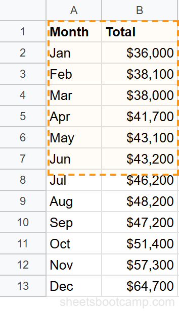
We’ll use the monthly summary data with Month in column A and Total in column B.

Start with a chart that uses a fixed range. In this example, the chart reads A1:B7 and displays a line chart of January through June. Rows 8-13 contain July through December, but the chart ignores them.

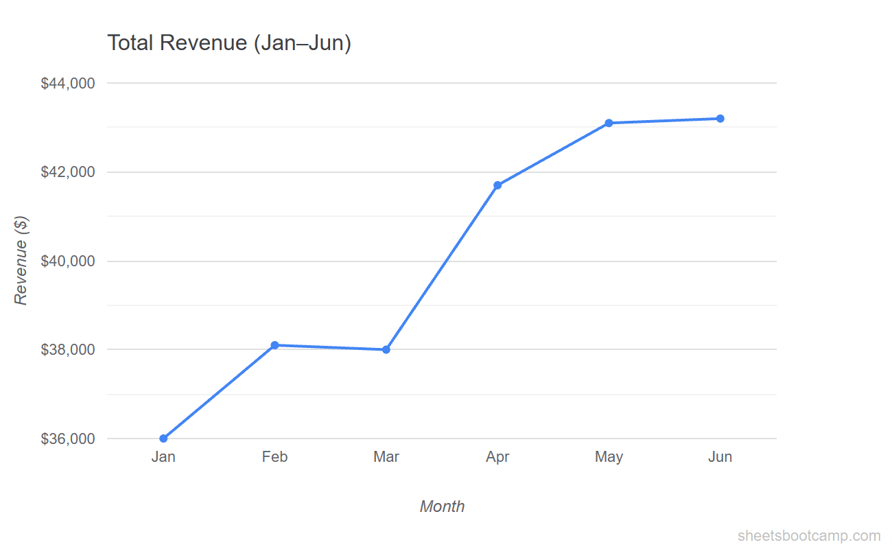
The chart shows six data points. The remaining six months of data sit in the spreadsheet, invisible to the chart.

Go to Data > Named ranges. In the sidebar that opens:

1. Enter a name: SalesData
2. Set the range to A1:B13 (all 12 months plus the header row)
3. Click Done

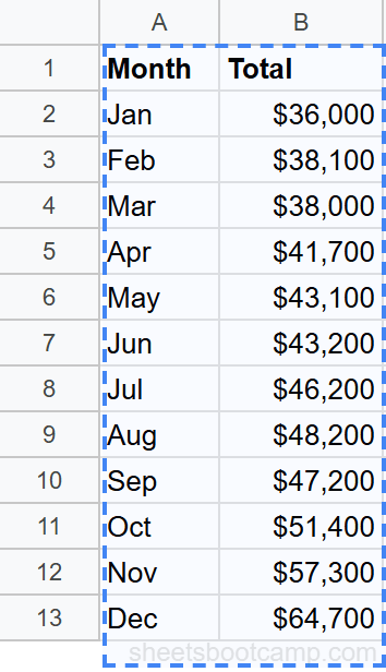
The named range now acts as an alias for A1:B13. Any formula or chart that references “SalesData” reads all 12 rows.

Double-click the chart to open the Chart Editor. In the Setup tab, click the Data range field. Delete the fixed range (A1:B7) and type SalesData in its place.

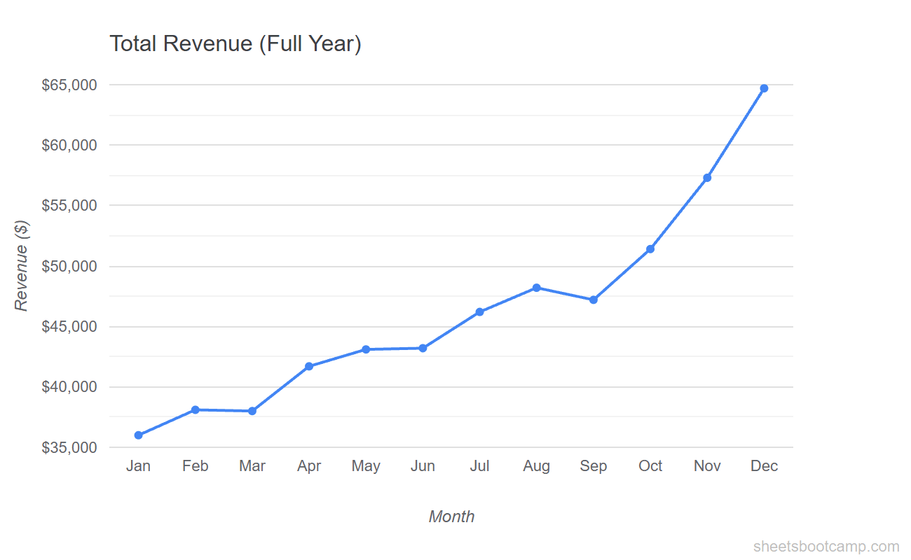
Google Sheets resolves the name to A1:B13 and the chart now reads all 12 months of data.

The chart now shows all 12 months, from January through December.

To add more data in the future (for example, a second year starting in row 14), update the named range under Data > Named ranges to extend through the new rows. Every chart that uses SalesData picks up the change.

Whole-Column References

The fastest way to make a chart dynamic is to reference entire columns instead of a specific range.

Instead of A1:B13, set the chart data range to A:B. Google Sheets scans all of column A and column B, including every non-empty cell. When you add row 14, 15, or 100, the chart includes them automatically.

How to set it up:

1. Double-click the chart to open the Chart Editor
2. In the Data range field, replace the fixed range with A:B
3. The chart now reads every row in columns A and B that contains data

Advantages:

• No named range to maintain
• No formulas needed
• Works immediately for any number of new rows

Disadvantages:

• Scans the entire column (over 1,000,000 rows), which can slow down large sheets
• Picks up any stray data in those columns, including notes or test values below your table
• Does not work if you have unrelated data further down in the same columns

OFFSET Formula for Dynamic Ranges

OFFSET creates a range that starts at a specific cell and extends by a calculated number of rows. Combined with COUNTA (which counts non-empty cells), OFFSET builds a range that grows and shrinks with your data.

The formula for a dynamic single-column range:

=OFFSET(A1, 0, 0, COUNTA(A:A), 1)

This starts at cell A1, moves 0 rows down and 0 columns over, then extends for COUNTA(A:A) rows and 1 column. If column A has 13 non-empty cells (1 header + 12 months), OFFSET returns the range A1:A13. Add a 13th month and it returns A1:A14.

For a two-column range (Month + Total):

=OFFSET(A1, 0, 0, COUNTA(A:A), 2)

The last argument changes from 1 to 2, which makes the range span two columns (A and B).

How to use OFFSET with a chart:

Google Sheets does not accept OFFSET directly in the Chart Editor data range field. You need to wrap it in a named range:

1. Go to Data > Named ranges
2. Name it DynamicSales
3. In the range field, enter: =OFFSET(Sheet1!A1, 0, 0, COUNTA(Sheet1!A:A), 2)
4. Use DynamicSales as the chart data range

The OFFSET method is the most flexible of the three approaches. It handles gaps, partial data, and multi-column ranges. The trade-off is added complexity. If the whole-column method works for your data, it is the faster option.

Tips and Best Practices

1. Start with whole-column references for small datasets. If your sheet has fewer than a few hundred rows and the columns are dedicated to chart data, A:B is the fastest setup with no maintenance.

2. Use named ranges when multiple charts share the same data. Update the named range once and every chart that references it picks up the change. This is especially useful in dashboards.

3. Add OFFSET when you need precision. OFFSET with COUNTA gives you exact control over how many rows the range includes. Use it when whole-column references pick up unwanted data.

4. Keep chart data in dedicated columns. Mixing chart data with other content in the same column causes all three methods to break. Isolate your chart source data in its own block of columns.

5. Test after adding new rows. After entering new data, check that the chart updated. If it did not, verify the named range definition or column reference in the Chart Editor. A typo in the range name is the most common cause of charts not updating.

Related Google Sheets Tutorials

• Google Sheets Charts: The Complete Guide — Overview of all chart types with creation and customization basics
• How to Make a Line Chart — Show trends over time with line charts and trendlines
• How to Make a Bar Chart — Compare values across categories with horizontal bars
• How to Make a Pie Chart — Display proportions and category breakdowns in a circle chart

Frequently Asked Questions

How do I make a chart auto-update in Google Sheets?

Use a named range, a whole-column reference (like A:A), or an OFFSET formula as the chart data source. When you add new rows, the chart includes them automatically without manual range edits.

Can I use a named range as a chart data source?

Yes. Define a named range under Data > Named ranges, then type the name into the chart’s data range field in the Chart Editor. When you expand the named range to include new rows, the chart updates.

What is the easiest way to make a dynamic chart?

Reference entire columns like A:A instead of a fixed range like A1:A13. Google Sheets includes all non-empty cells in that column. This works well for small to medium datasets.

Does using whole-column references slow down charts?

On large sheets with thousands of rows, whole-column references can slow down chart rendering because Sheets scans the entire column. For large datasets, use a named range or OFFSET formula that targets only the data rows.

How does OFFSET work for dynamic chart ranges?

OFFSET returns a range that starts at a given cell and extends by a calculated number of rows. Use =OFFSET(A1,0,0,COUNTA(A:A),1) to create a range that grows with your data. Define this as a named range and use it as the chart source.