
QUERY filters, sorts, and summarizes data with one formula: =QUERY(data, query, [headers]), where the query is a quoted string of SQL-like clauses. Example: =QUERY(A1:G11, "SELECT B, D, F WHERE F > 400") returns the 3 sales rows with revenue over $400, headers included.
beginner 9 min read
Google Sheets QUERY Function: Complete Guide
Learn how to use the QUERY function in Google Sheets to filter, sort, and summarize data. Step-by-step examples with SELECT, WHERE, and GROUP BY.
SB
Sheets Bootcamp
February 18, 2026 · Updated August 13, 2026
Table of Contents
Quick Answer
The QUERY function in Google Sheets filters, sorts, and summarizes data using a text-based query language borrowed from SQL. You write conditions in a quoted string, and QUERY returns the matching rows. It’s one of the most flexible functions in Sheets, a single formula can do what normally takes FILTER, SORT, and a pivot table combined.
This guide covers the QUERY syntax, walks through real examples with sales data, and shows how to use SELECT, WHERE, GROUP BY, and other clauses.
In This Guide
- QUERY Function Syntax
- How to Use QUERY in Google Sheets: Step-by-Step
- QUERY Clause Reference
- QUERY Examples
- QUERY Across Multiple Sheets
- Common QUERY Errors
- Tips and Best Practices
- Related Google Sheets Tutorials
- FAQ
QUERY Function Syntax
Watch the three arguments explained (1:11)
The QUERY function takes three arguments:
Formula
=QUERY(data, query, [headers]) | Parameter | Description | Required |
|---|---|---|
| data | The range of cells to query (e.g., A1:G18) | Yes |
| query | A text string written in Google’s query language (e.g., "SELECT A, B WHERE C > 10") | Yes |
| headers | The number of header rows in your data. Defaults to a best guess. | No |
The query string uses the Google Visualization API Query Language. It borrows keywords from SQL, SELECT, WHERE, GROUP BY, ORDER BY, but it is not full SQL. The biggest difference: you reference columns by letter (A, B, C), not by header name.
Important
Inside the query string, columns are referenced by their letter in the data range. If your data starts in column A, then column A in the query is the first column of your data. If your range starts at column D, then column D in the query maps to the first column. Always match column letters to where your data actually starts.
How to Use QUERY in Google Sheets: Step-by-Step
We’ll use a sales records table to pull specific columns and filter rows based on revenue.
Sample Data
1
Identify your data range
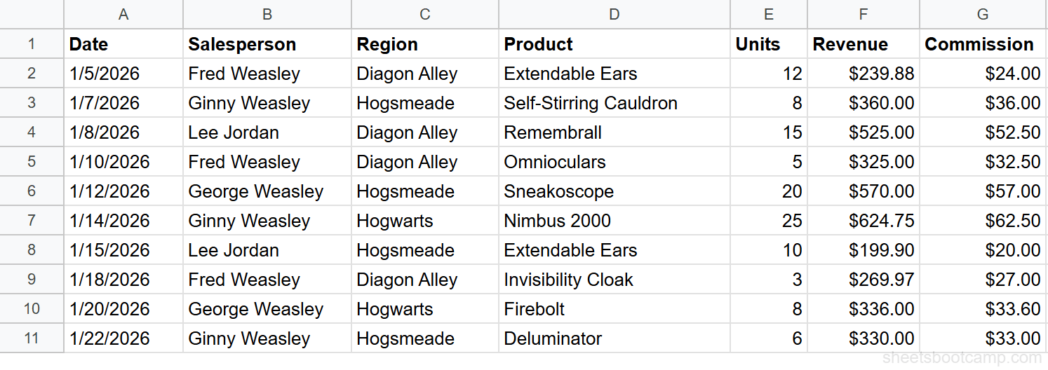
You need a range with a header row and consistent data below it. In this table, A1:G11 covers the headers plus 10 data rows. The columns are Date (A), Salesperson (B), Region (C), Product (D), Units (E), Revenue (F), and Commission (G).
2
Write a SELECT query
Select an empty cell and enter:
Formula
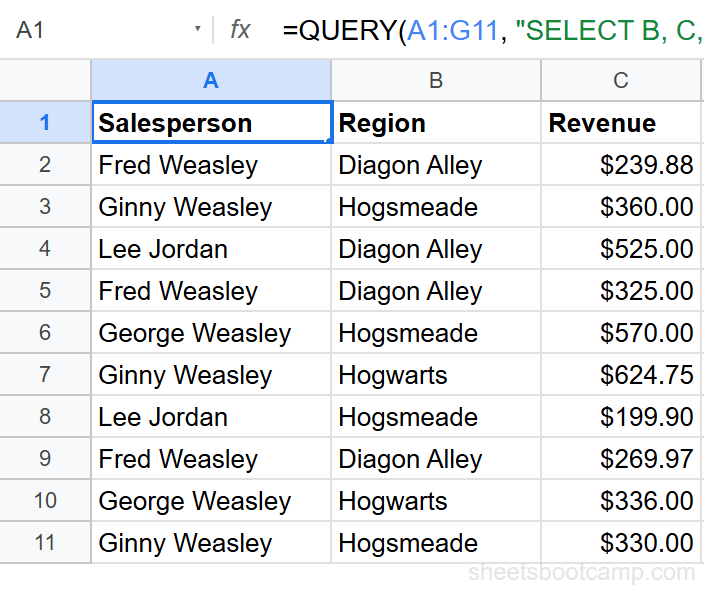
=QUERY(A1:G11, "SELECT B, C, F") This pulls three columns from the data: Salesperson (B), Region (C), and Revenue (F). QUERY returns a new table with just those columns, including the header row.
3
Add a WHERE filter
Modify the formula to include a condition:
Formula
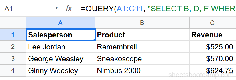
=QUERY(A1:G11, "SELECT B, D, F WHERE F > 400") This returns only the rows where Revenue (column F) exceeds $400. The result shows the Salesperson, Product, and Revenue for each qualifying sale.
4
Review the result set
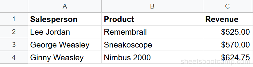
QUERY returns a complete table, headers and matching data rows. For this query, you get 3 rows: Inspector Lestrade’s Pocket Watch ($525.00), Mycroft Holmes’s Cipher Decoder ($570.00), and Irene Adler’s Magnifying Glass ($624.75).
Tip
QUERY results spill into adjacent cells automatically. Make sure the cells below and to the right of your formula are empty, or QUERY returns a #REF! error.
QUERY Clause Reference
The query string supports several clauses. You can combine them in a single formula, but they must appear in this order: SELECT, WHERE, GROUP BY, PIVOT, ORDER BY, LIMIT, OFFSET, LABEL, FORMAT.
SELECT
Watch SELECT choose columns (2:37)
Chooses which columns to return. Use * for all columns, or list specific column letters separated by commas.
Formula
=QUERY(A1:G11, "SELECT B, D, F") Returns only Salesperson, Product, and Revenue. For more patterns, see the QUERY SELECT guide.
WHERE
Watch WHERE filter rows (3:44)
Filters rows based on a condition. Works with comparison operators (=, !=, >, <, >=, <=), text matching (contains, starts with, ends with, matches), and IS NULL / IS NOT NULL.
Formula
=QUERY(A1:G11, "SELECT * WHERE C = 'Scotland Yard'") Returns all columns, but only rows where Region is “Scotland Yard”. Text values inside WHERE must be wrapped in single quotes. For a complete walkthrough, see the QUERY WHERE guide.
GROUP BY
Watch GROUP BY and PIVOT build totals (5:32)
Groups rows by a column and applies aggregate functions: SUM, COUNT, AVG, MIN, MAX.
Formula
=QUERY(A1:G11, "SELECT C, SUM(F) GROUP BY C") Returns one row per region with the total revenue for each. See the QUERY GROUP BY guide for more aggregation patterns.
PIVOT
Turns the values of a column into result columns, one per unique value, and aggregates into the cells. It is a pivot table in a single clause.
Formula
=QUERY(A1:G11, "SELECT SUM(F) PIVOT C") Returns one row with a column per region, each holding that region’s total revenue: Baker Street $1,359.85, Scotland Yard $1,459.90, Whitehall $960.75. Combine it with GROUP BY to get rows and columns at once, for example "SELECT B, SUM(F) GROUP BY B PIVOT C" totals every salesperson by region. See the QUERY PIVOT guide for the full pattern.
ORDER BY
Watch ORDER BY, LIMIT and LABEL (7:20)
Sorts the result set by one or more columns. Add ASC (ascending, default) or DESC (descending).
Formula
=QUERY(A1:G11, "SELECT B, F ORDER BY F DESC") Returns all rows sorted by Revenue from highest to lowest. See the QUERY ORDER BY guide for multi-column sorts.
LIMIT
Restricts the number of rows returned.
Formula
=QUERY(A1:G11, "SELECT B, F ORDER BY F DESC LIMIT 3") Returns only the top 3 rows by revenue.
LABEL
Renames column headers in the result.
Formula
=QUERY(A1:G11, "SELECT C, SUM(F) GROUP BY C LABEL SUM(F) 'Total Revenue'") The aggregated column header changes from “sum Revenue” to “Total Revenue”. See the QUERY LABEL guide for renaming several columns at once.
Note
You can chain multiple clauses in a single query string. They must follow the order: SELECT, WHERE, GROUP BY, PIVOT, ORDER BY, LIMIT, OFFSET, LABEL, FORMAT. Putting them out of order causes a parsing error.
QUERY Examples
Example 1: Filter by Text Match
You want to see all sales made by Irene Adler.
Formula
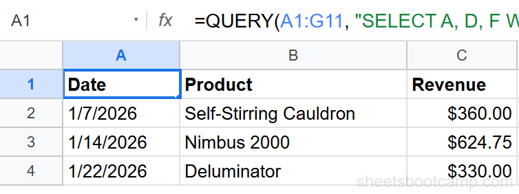
=QUERY(A1:G11, "SELECT A, D, F WHERE B = 'Irene Adler'") This returns 3 rows from the first 10 data rows: Scotland Yard Forensic Chemistry Set ($360.00), Whitehall Magnifying Glass ($624.75), and Scotland Yard Lockpick Set ($330.00). The query checks column B (Salesperson) for an exact text match.
Important
Text values in WHERE clauses must be wrapped in single quotes: 'Irene Adler', not double quotes. The outer formula already uses double quotes, so single quotes avoid conflicts. Text matching is case-sensitive, 'sherlock holmes' returns no results.
Example 2: Aggregate with GROUP BY
You want total revenue by region.
Formula
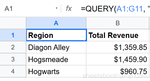
=QUERY(A1:G11, "SELECT C, SUM(F) GROUP BY C LABEL SUM(F) 'Total Revenue'") This returns 3 rows, one for each region, with the summed revenue:
| Region | Total Revenue |
|---|---|
| Baker Street | $1,359.85 |
| Scotland Yard | $1,459.90 |
| Whitehall | $960.75 |
The LABEL clause renames the aggregated column from the default “sum Revenue” to “Total Revenue”.
Example 3: Combined Clauses
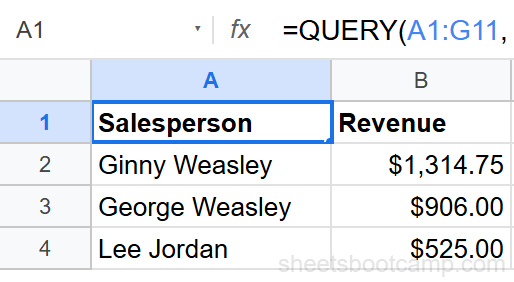
You want the top 3 salespeople by total revenue, but only for sales over $300.
Formula
=QUERY(A1:G11, "SELECT B, SUM(F) WHERE F > 300 GROUP BY B ORDER BY SUM(F) DESC LIMIT 3 LABEL SUM(F) 'Revenue'") This chains five clauses: SELECT picks the Salesperson and aggregated Revenue. WHERE filters out sales under $300. GROUP BY totals each person’s qualifying sales. ORDER BY sorts highest first. LIMIT keeps only the top 3.
QUERY Across Multiple Sheets
Watch two sheets stacked, then IMPORTRANGE (9:54)
Stack ranges inside curly braces to query them as one table. Separate the ranges with semicolons, and give every range the same number of columns:
Formula
=QUERY({Jan!A2:G11; Feb!A2:G11}, "SELECT Col2, Col6 WHERE Col6 > 400", 0) Two things change when you stack ranges. First, start the ranges below the header row (A2, not A1) and set the third argument to 0, or the second sheet’s header row lands in the middle of your data. Second, column letters stop working: the stacked table is a new array that no longer lives on the sheet, so you refer to its columns by position as Col1, Col2, Col3. SELECT B errors on a stacked range; SELECT Col2 returns its second column.
The same Col1 notation applies when the data argument is a function result instead of a plain range, which is exactly what happens with IMPORTRANGE:
Formula
=QUERY(IMPORTRANGE("spreadsheet_url", "Sheet1!A1:G"), "SELECT Col2, Col6", 1) For the full walkthrough, see QUERY multiple ranges and QUERY with IMPORTRANGE.
Common QUERY Errors
Watch all four ways it breaks (11:24)
Parsing Error
The most common QUERY error. You see a message like: Unable to parse query string for Function QUERY parameter 2.
This happens when:
- A clause is misspelled (
SLECTinstead ofSELECT) - Clauses are out of canonical order. The order is SELECT, WHERE, GROUP BY, PIVOT, ORDER BY, LIMIT, OFFSET, LABEL, FORMAT, with no exceptions:
WHEREbeforeSELECTerrors, and so doesORDER BYbeforeWHERE - Text values are missing single quotes:
WHERE B = Sherlock Holmesinstead ofWHERE B = 'Sherlock Holmes' - Column letters don’t exist in the data range
Fix it by checking the query string character by character. The error message sometimes includes the position where parsing stopped.
Cells That Silently Go Blank
QUERY expects each column to contain one data type. If a column has a mix of numbers and text, QUERY uses the majority type, and every cell holding the minority type comes back blank. The row itself survives: on a numeric column with one text entry, SELECT still returns all the rows, but that one cell arrives empty. SUM on the same column skips the text value and totals the rest, again with no error.
This commonly happens when a numeric column contains text entries like “N/A” or “Pending” mixed in with numbers. Clean the data first, or use a separate column with a formula to handle the conversion.
Warning
QUERY silently blanks cells when a column has mixed data types. You won’t get an error, and the row count still looks right, so nothing tips you off. If a QUERY result has holes in a column, check the source column for mixed text and numbers.
Wrong Header Count
If the headers parameter (third argument) is wrong, QUERY might treat data rows as headers or vice versa.
Formula
=QUERY(A1:G11, "SELECT B, F", 1) Setting headers to 1 explicitly tells QUERY the first row is a header. If you omit this parameter, QUERY guesses, and it usually guesses correctly. But when your data starts below row 1 or has multiple header rows, set it explicitly.
Date Handling
Watch the date keyword everyone forgets (8:43)
Dates in QUERY WHERE clauses need a special format:
Formula
=QUERY(A1:G11, "SELECT * WHERE A > date '2026-01-15'") Use the date keyword followed by the date in 'YYYY-MM-DD' format inside single quotes. Without the date keyword, QUERY treats the value as text and the comparison breaks. See the QUERY dates guide for filtering by month, year, and rolling windows.
Tips and Best Practices
-
Use column letters, not header names. Inside the query string,
Frefers to sheet column F, which must be inside your range. Header names don’t work. If your range isC1:H10, thenCin the query refers to the first column of that range. -
Wrap text values in single quotes.
WHERE B = 'Scotland Yard'works.WHERE B = "Scotland Yard"breaks because the double quotes collide with the formula’s outer quotes. -
Set the headers parameter explicitly. Adding
1as the third argument (=QUERY(A1:G11, "SELECT *", 1)) removes ambiguity. QUERY’s auto-detection works most of the time, but explicit is safer. -
Use FILTER for simple row filtering. If you only need to return rows matching a condition without sorting, grouping, or reshaping, FILTER is faster to write and easier to read. Reserve QUERY for when you need multiple clauses.
-
Combine with IMPORTRANGE for cross-spreadsheet queries.
=QUERY(IMPORTRANGE("url", "Sheet1!A1:G"), "SELECT *")lets you query data from a different file. See the QUERY with IMPORTRANGE guide for setup details.
Tip
When debugging a QUERY formula, start with "SELECT *" to return everything, then add one clause at a time. This makes it easy to find which clause causes the error.
Related Google Sheets Tutorials
- QUERY WHERE Clause: Filter rows using conditions, comparisons, and text matching
- QUERY SELECT: Choose specific columns and reorder them in the output
- QUERY GROUP BY: Aggregate data with SUM, COUNT, AVG, and other functions
- QUERY PIVOT: Turn column values into result columns, a pivot table in one clause
- QUERY ORDER BY: Sort results by one or more columns
- QUERY LABEL: Rename result headers, including aggregated columns
- QUERY Date Filters: Filter by day, month, year, and rolling date windows
- QUERY Multiple Ranges: Stack sheets with curly braces and the Col1 notation
- QUERY with IMPORTRANGE: Query data that lives in a different spreadsheet file
- IF Function Guide: Conditional logic for evaluating true/false conditions per row
- VLOOKUP Complete Guide: Look up values from a table, useful when you need a single value instead of a filtered dataset
Frequently Asked Questions
What does the QUERY function do in Google Sheets?
QUERY filters, sorts, and summarizes data using a text-based query language similar to SQL. You write conditions like SELECT, WHERE, and GROUP BY inside a quoted string, and QUERY returns the matching rows and columns.
What language does QUERY use in Google Sheets?
QUERY uses the Google Visualization API Query Language. It borrows concepts from SQL (SELECT, WHERE, GROUP BY, ORDER BY) but is not full SQL. Column references use letters (A, B, C) instead of column names.
How do you filter rows with QUERY in Google Sheets?
Add a WHERE clause to your query string. For example, =QUERY(A1:G18, "SELECT * WHERE F > 400") returns only rows where column F exceeds 400. Use single quotes for text values: WHERE B = 'Irene Adler'.
Can you use QUERY with data from another sheet?
Yes. Reference the other sheet in the data argument: =QUERY('Sheet2'!A1:G18, "SELECT B, F"). You can also combine QUERY with IMPORTRANGE to pull data from a different spreadsheet file entirely.
What is the difference between QUERY and FILTER in Google Sheets?
FILTER returns rows that match a condition and is faster for simple filtering. QUERY can also sort, group, aggregate, limit, and relabel results in a single formula. Use FILTER for quick row filtering and QUERY when you need to reshape or summarize the data.
How do you QUERY multiple sheets at once?
Stack the ranges inside curly braces, separated by semicolons: =QUERY({Jan!A2:G11; Feb!A2:G11}, "SELECT Col2, Col6", 0). Inside a stacked range, column letters stop working, so refer to columns as Col1, Col2, Col3 in order.
You've googled this formula before. Probably more than once.
The Bootcamp is a real Google Sheet that grades every formula the moment you press Enter. 193 exercises across 9 modules, the 10% of Sheets that does 90% of the work. One payment of $29.
Get It for $29 Get the Bootcamp for $2930-day refund. Reply to any email and you get your money back.
Not ready to pay? Try Basic Training free →