
IF tests a condition and returns one value when it is true and another when it is false: =IF(logical_expression, value_if_true, value_if_false). Example: =IF(F2>400, "Bonus", "No Bonus") returns Bonus for any sale over $400 and No Bonus for the rest.
beginner 7 min read
Google Sheets IF Function: Complete Guide
Learn how to use the IF function in Google Sheets with step-by-step examples. Covers syntax, nested IF, IF with AND/OR, common errors, and best practices.
SB
Sheets Bootcamp
February 18, 2026 · Updated August 17, 2026
Table of Contents
Quick Answer
The IF function in Google Sheets tests a condition and returns different values based on whether that condition is true or false. It’s the foundation of every logical formula in Sheets, once you understand IF, functions like COUNTIF, SUMIF, and IFS all make more sense.
This guide covers the IF function syntax, walks through real examples with sales data, and shows how to combine IF with AND, OR, and nested conditions.
In This Guide
- IF Function Syntax
- How to Use IF in Google Sheets: Step-by-Step
- IF Function Examples
- Nested IF Statements
- IF with AND and OR
- Common IF Function Errors
- Tips and Best Practices
- Related Google Sheets Tutorials
- FAQ
IF Function Syntax
The IF function takes three arguments:
Formula
=IF(logical_expression, value_if_true, value_if_false) | Parameter | Description | Required |
|---|---|---|
| logical_expression | A condition that evaluates to TRUE or FALSE (e.g., A1>100, B2="Yes") | Yes |
| value_if_true | The value returned when the condition is TRUE | Yes |
| value_if_false | The value returned when the condition is FALSE | No |
The condition can use any comparison operator:
| Operator | Meaning | Example |
|---|---|---|
= | Equal to | A1="Yes" |
<> | Not equal to | A1<>"" |
> | Greater than | B2>100 |
< | Less than | B2<50 |
>= | Greater than or equal to | C3>=90 |
<= | Less than or equal to | C3<=0 |
Important
If you omit value_if_false, the function returns FALSE (the boolean value, not the text “FALSE”). To return a blank cell instead, use an empty string: =IF(A1>100, "Over", "").
How to Use IF in Google Sheets: Step-by-Step
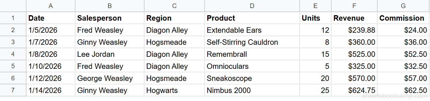
We’ll use a sales records table to determine which transactions qualify for a bonus. Any sale with revenue over $400 earns a bonus.
Watch this formula built and filled down a column (1:09)
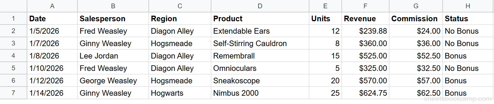
Sample Data
1
Set up your data
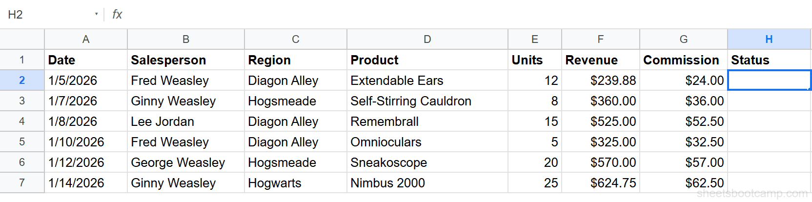
You need a column with values to evaluate. In this table, column F (Revenue) contains the values we’ll check. Select cell H2, that’s where the IF result will go.
2
Enter the IF formula
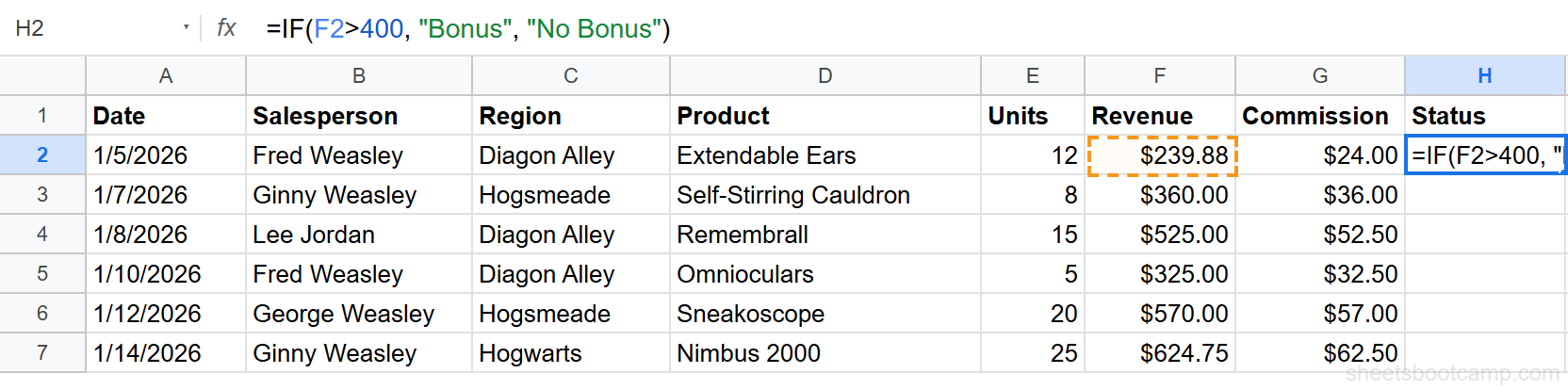
Type the following formula in cell H2:
Formula
=IF(F2>400, "Bonus", "No Bonus") This checks whether the revenue in F2 is greater than 400. If true, it returns “Bonus”. If false, it returns “No Bonus”.
3
Review the result
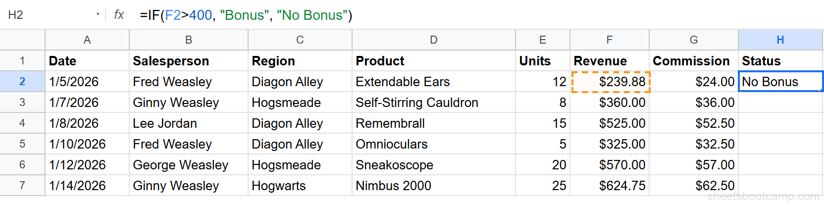
Press Enter. Cell H2 shows “No Bonus” because F2 contains $239.88, which is less than 400.
4
Copy the formula down the column
Select H2 and drag the fill handle down through H7. Each row evaluates its own revenue value. Rows with revenue over $400 show “Bonus” and the rest show “No Bonus”.
Tip
When copying IF formulas down a column, the cell references update automatically. F2 becomes F3, F4, and so on. If you need to reference a fixed cell (like a threshold value in a specific cell), use an absolute reference: $B$1.
IF Function Examples
Example 1: Label Performance Tiers
You want to label each sale as “Top Seller” when revenue exceeds $500, or “Standard” otherwise.
Formula
=IF(F2>500, "Top Seller", "Standard") For row 7 where Irene Adler sold a Magnifying Glass for $624.75, this returns “Top Seller”. For row 2 where Sherlock Holmes sold a Listening Device for $239.88, it returns “Standard”.
Example 2: Check for Empty Cells
Before running calculations on a column, you might need to check whether cells contain data.
Formula
=IF(A2="", "Missing", A2) If cell A2 is empty, this returns “Missing”. If A2 has a value, it returns that value as-is. This is useful for flagging incomplete records in a shared spreadsheet.
Note
An empty string "" and a blank cell are not the same thing in Google Sheets. A cell that looks empty might contain a space or a zero-length formula result. Use =IF(ISBLANK(A2), "Empty", "Has data") to specifically test for truly blank cells.
Example 3: Return a Calculated Value
IF doesn’t have to return text. It can return numbers, formulas, or calculations.
Formula
=IF(E2>10, F2*0.1, F2*0.05) This creates a tiered commission: 10% commission on sales with more than 10 units, and 5% on smaller sales. For row 4 where Inspector Lestrade sold 15 Pocket Watches for $525.00, this returns $52.50 (10% rate). For row 5 where Sherlock Holmes sold 5 Field Binoculars for $325.00, it returns $16.25 (5% rate).
Nested IF Statements
When you need more than two outcomes, nest one IF inside another. Each IF handles one condition, and the false branch passes control to the next IF.
Watch tiers built with a nested IF (3:37)
Formula
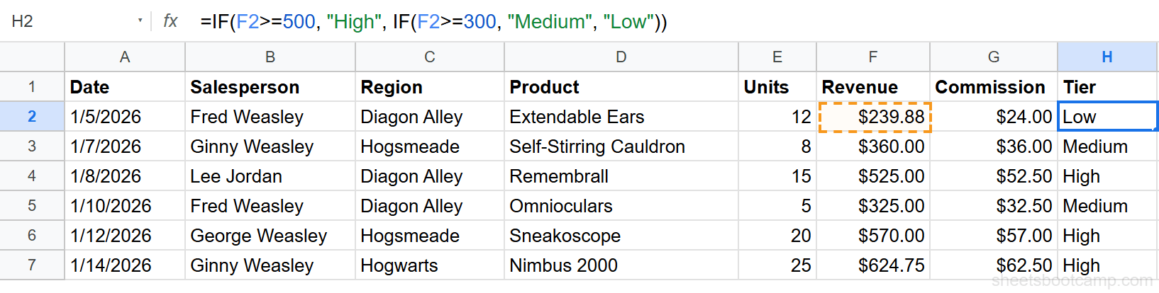
=IF(F2>=500, "High", IF(F2>=300, "Medium", "Low")) This creates three tiers:
- Revenue $500 or more → “High”
- Revenue $300 to $499 → “Medium”
- Revenue under $300 → “Low”
For Irene Adler’s $624.75 Magnifying Glass sale, this returns “High”. For Sherlock Holmes’s $239.88 Listening Device sale, it returns “Low”.
Note
Nested IFs get hard to read after 3 levels. For 4 or more conditions, use the IFS function instead. IFS checks multiple conditions in a flat list without nesting.
For a deeper walkthrough with more complex examples, see our guide on nested IF statements in Google Sheets.
IF with AND and OR
Combine IF with AND or OR to test multiple conditions at once.
Watch AND and OR inside one IF (6:27)
IF with AND (all conditions must be true)
AND returns TRUE only when every condition inside it is true.
Formula
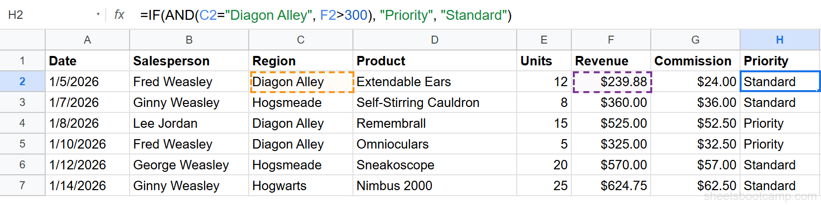
=IF(AND(C2="Baker Street", F2>300), "Priority", "Standard") This checks two things: the region is Baker Street AND revenue exceeds $300. Both must be true to return “Priority”. For Sherlock Holmes’s $325.00 Field Binoculars sale in Baker Street, this returns “Priority”. For his $239.88 Listening Device sale (also Baker Street but under $300), it returns “Standard”.
IF with OR (any condition can be true)
OR returns TRUE when at least one condition is true.
Formula
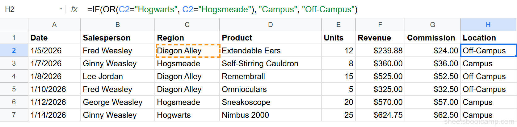
=IF(OR(C2="Whitehall", C2="Scotland Yard"), "Campus", "Off-Campus") This checks whether the region is Whitehall OR Scotland Yard. Either one returns “Campus”. Any other region returns “Off-Campus”. For Irene Adler’s Whitehall sale, this returns “Campus”. For Sherlock Holmes’s Baker Street sale, it returns “Off-Campus”.
For more patterns including combined AND/OR conditions, see the full guide on IF with AND and OR.
Common IF Function Errors
Watch the three ways the condition lies to you (2:10)
Watch IFERROR catch what is left (10:01)
Empty String vs. FALSE
If you write =IF(A1>100, "Yes") without a third argument, the false result is the boolean value FALSE, not a blank cell. This can break formulas that reference the cell later.
Fix it by always including the third argument:
Formula
=IF(A1>100, "Yes", "") The empty string "" displays as a blank cell and doesn’t interfere with other formulas.
Text in a Number Comparison Passes Silently
Comparing text to a number does not error, and that is the trap. Google Sheets sorts every text value above every number, so the comparison quietly comes out TRUE:
Formula
=IF("hello">100, "Yes", "No") This returns “Yes”, with no error. In real data that behavior is dangerous: one text entry like “Pending” or “N/A” in a numeric column makes every > test on that cell pass. A sanity check with MAX will not catch it either, because MAX skips text entirely.
To guard a numeric test against text, require a number as part of the condition:
Formula
=IF(AND(ISNUMBER(F2), F2>400), "Bonus", "No Bonus") #VALUE! Error
Arithmetic on text is what actually errors. ="hello"+100 returns #VALUE!, and so does any IF whose condition or result branch does math on a text value. If an IF formula shows #VALUE!, look for a calculation touching a cell that holds text, not for a comparison.
Text Comparisons Are Not Case-Sensitive
=IF(A1="apple", "Found", "Not found") returns “Found” for “apple”, “APPLE”, and “Apple”. IF treats all three as equal.
If you need case-sensitive matching:
Formula
=IF(EXACT(A1, "Apple"), "Match", "No match") The EXACT function compares two strings with case sensitivity, and the IF function acts on the result.
Comparing Dates
Dates in Google Sheets are numbers. You can compare them directly:
Formula
=IF(A2>DATE(2026,1,15), "After Jan 15", "Before Jan 15") Use the DATE function to create a date value for comparison. Don’t compare against a text string like “1/15/2026”, it will work sometimes but fail when date formats differ.
Tip
Wrap any IF formula in IFERROR to catch unexpected errors: =IFERROR(IF(F2>400, "Bonus", "No Bonus"), "Check data"). This prevents a single bad cell from breaking an entire column of formulas.
Tips and Best Practices
-
Always include the third argument. Omitting
value_if_falsereturns the booleanFALSE, which displays as “FALSE” in the cell and confuses other formulas. Use""for a blank cell or0for zero. -
Keep nesting under 3 levels.
=IF(A, X, IF(B, Y, IF(C, Z, W)))is about as deep as you should go. Beyond that, switch to IFS or SWITCH. -
IF is not case-sensitive. For case-sensitive text checks, wrap the condition in
EXACT(). -
Use absolute references when copying down. If your formula references a fixed threshold (like a target in cell B1), lock it with
$B$1so it doesn’t shift when you drag the formula down. -
Combine with IFERROR for cleaner results.
=IFERROR(IF(...), "Error")catches any unexpected issues and returns a clean fallback value.
Related Google Sheets Tutorials
- Nested IF Statements in Google Sheets: Handle 3 or more outcomes by stacking IF functions inside each other
- IFS Function in Google Sheets: Check multiple conditions without nesting, cleaner than nested IF for 4+ outcomes
- IF with AND / OR in Google Sheets: Test multiple conditions at once using AND (all must be true) or OR (any can be true)
- COUNTIF and COUNTIFS Guide: Count cells that match one or more conditions
- SUMIF and SUMIFS Guide: Add up values that match specific criteria
- IFERROR in Google Sheets: Catch errors and return a clean fallback value
- SWITCH Function Guide: Compare one value against a list of cases, cleaner than nested IF for exact matches
- IF with Checkboxes: Drive formulas from TRUE/FALSE checkbox values
- VLOOKUP Complete Guide: Look up values from a table, often combined with IF for conditional lookups
Frequently Asked Questions
What does the IF function do in Google Sheets?
The IF function tests a condition and returns one value when the condition is true and a different value when it is false. For example, =IF(A1>100, "Over budget", "Within budget") checks if A1 exceeds 100 and returns the matching label.
How do you write an IF/THEN formula in Google Sheets?
Use the syntax =IF(condition, value_if_true, value_if_false). The condition is any expression that evaluates to TRUE or FALSE. For example, =IF(B2="Yes", "Complete", "Pending") checks if B2 contains "Yes" and returns the appropriate status.
Can you nest IF statements in Google Sheets?
Yes. Place another IF function inside the value_if_true or value_if_false argument. For example, =IF(A1>=90, "A", IF(A1>=80, "B", "C")) checks multiple conditions in sequence. Google Sheets supports nesting, but beyond 3 levels, IFS is cleaner.
Is the IF function case-sensitive in Google Sheets?
No. IF treats "apple" and "APPLE" as the same value when comparing text. If you need a case-sensitive comparison, wrap the condition in EXACT: =IF(EXACT(A1, "Apple"), "Match", "No match").
What is the difference between IF and IFS in Google Sheets?
IF checks one condition and returns one of two values. IFS checks multiple conditions in order and returns the value for the first true condition. IFS replaces deeply nested IF statements with a flat, readable formula.
Can you use an IF formula in conditional formatting?
Yes, through the custom formula option, but you do not wrap it in IF. Conditional formatting only needs the condition itself, so a rule like =$F2>400 highlights every row where revenue exceeds 400. The IF wrapper is only needed in cells, where a formula must return a value.
You've googled this formula before. Probably more than once.
The Bootcamp is a real Google Sheet that grades every formula the moment you press Enter. 193 exercises across 9 modules, the 10% of Sheets that does 90% of the work. One payment of $29.
Get It for $29 Get the Bootcamp for $2930-day refund. Reply to any email and you get your money back.
Not ready to pay? Try Basic Training free →