
To count the days between two dates in Google Sheets, subtract them: =B2-A2. For complete years use =DATEDIF(A2, B2, "Y"), to shift a date by months use =EDATE(A2, 6), and for business days use =NETWORKDAYS(A2, B2). Every date is stored as a serial number (February 18, 2026 is 46071), which is why date math works at all.
beginner 13 min read
Date Functions in Google Sheets: Complete Guide
Learn how to use date functions in Google Sheets to calculate age, tenure, deadlines, and business days. Examples with TODAY, DATEDIF, EDATE, and more.
SB
Sheets Bootcamp
February 18, 2026 · Updated August 17, 2026
Table of Contents
Quick Answer
Date functions in Google Sheets let you calculate age, tenure, deadlines, and time differences using formulas that understand dates. Whether you need the number of business days between two dates or want to add six months to a hire date, Sheets has a function for it.
Dates in Google Sheets are numbers wearing a disguise. Understanding that one concept makes every date formula in this guide easier.
We’ll cover the core date functions with syntax and examples, walk through calculating employee tenure step by step, and fix the errors that trip people up most often.
In This Guide
- What Are Date Functions in Google Sheets?
- How Dates Work: The Serial Number System
- Essential Date Functions: Syntax and Examples
- How to Calculate Days Between Dates: Step-by-Step
- Date Function Examples
- Common Errors and How to Fix Them
- Tips and Best Practices
- Related Google Sheets Tutorials
- FAQ
What Are Date Functions in Google Sheets?
Date functions are built-in formulas that create, extract, and calculate with dates. Google Sheets includes over 20 date functions. Some return today’s date. Some calculate the difference between two dates. Others convert text to dates or add months to existing dates.
The most commonly used date functions:
- TODAY and NOW: return the current date or date-and-time
- DATE: build a date from separate year, month, and day values
- YEAR, MONTH, DAY: extract parts from an existing date
- DATEDIF: calculate the difference between two dates in years, months, or days
- EDATE and EOMONTH: shift a date forward or backward by a number of months
- NETWORKDAYS: count business days between two dates, excluding weekends
- DATEVALUE: convert a text string into a date Google Sheets can use in calculations
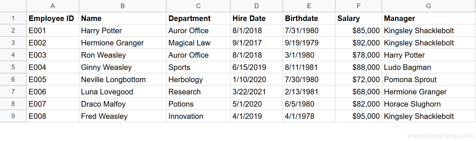
We’ll use an employee database throughout this guide. The table has 8 employees with hire dates, birthdates, and other fields that make date calculations practical.
How Dates Work: The Serial Number System
Google Sheets stores every date as a whole number called a serial number. Day zero is December 30, 1899, so January 1, 1900 is serial number 2, and today’s date is however many days have passed since that starting point.
This means February 18, 2026 is serial number 46071. July 31, 1980 (Sherlock Holmes’s birthdate in our data) is 29433.
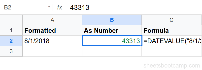
This serial number system is why date math works. Subtracting one date from another gives you the number of days between them. Adding 30 to a date moves it forward by 30 days. The date functions in this guide are built on top of this numbering system.
Important
If a cell displays a large number like 44927 instead of a date, the cell is formatted as a number. Select the cell, go to Format > Number > Date, and the date appears. The underlying value has not changed, only the display format. For more formatting options, see how to format dates in Google Sheets.
Times work the same way, but as decimal fractions. 0.5 represents noon (halfway through the day). A date-time like “February 18, 2026 6:00 PM” is stored as 46071.75. The date functions in this guide work with whole-number dates. Time functions are a separate topic.
Essential Date Functions: Syntax and Examples
TODAY and NOW
TODAY returns the current date. NOW returns the current date and time. Both update automatically whenever the spreadsheet recalculates.
Formula
=TODAY() Formula
=NOW() Neither function takes any arguments. TODAY returns a date like 7/6/2026. NOW returns a date-time like 7/6/2026 14:30:00. The exact value depends on when you open the sheet.
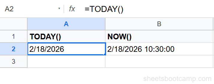
TODAY is the function you will use most often with date calculations. Combining it with DATEDIF lets you calculate someone’s current age or years of service without updating the formula manually. For a deeper look at both functions, see TODAY and NOW in Google Sheets.
DATE
DATE builds a date from three separate values: year, month, and day.
Formula
=DATE(year, month, day) | Parameter | Description | Required |
|---|---|---|
| year | The year (4 digits, e.g. 2026) | Yes |
| month | The month number (1-12) | Yes |
| day | The day of the month (1-31) | Yes |
Formula
=DATE(2026, 3, 15) This returns March 15, 2026. DATE is useful when year, month, and day values live in separate columns and you need to combine them into a single date for calculations.
DATE also handles overflow intelligently. =DATE(2026, 13, 1) returns January 1, 2027 because month 13 rolls into the next year. =DATE(2026, 1, 32) returns February 1, 2026 because day 32 of January rolls into February.
YEAR, MONTH, DAY
These three functions extract a single component from a date.
Formula
=YEAR(date) Formula
=MONTH(date) Formula
=DAY(date) Using Sherlock Holmes’s hire date (8/1/2018) in cell D2:
=YEAR(D2)returns 2018=MONTH(D2)returns 8=DAY(D2)returns 1
These functions are useful for grouping data by year or month, filtering records to a specific quarter, or building custom date displays. You can combine them with IF statements to create conditional logic based on date parts, for example, flagging employees hired before 2020.
For more extraction patterns and examples, see YEAR, MONTH, and DAY functions.
DATEDIF
DATEDIF calculates the difference between two dates in the unit you specify. It is one of the most useful date functions in Google Sheets, and the only one that counts whole years or whole months rather than days.
Formula
=DATEDIF(start_date, end_date, unit) | Parameter | Description | Required |
|---|---|---|
| start_date | The earlier date | Yes |
| end_date | The later date | Yes |
| unit | "Y" years, "M" months, "D" days, "YM" months after years, "MD" days after months, "YD" days after years | Yes |
Using Sherlock Holmes’s hire date (8/1/2018) and today’s date:
Formula
=DATEDIF(D2, TODAY(), "Y") This returns 7 (as of 2026), the number of complete years since Sherlock’s hire date.
Formula
=DATEDIF(D2, TODAY(), "YM") This returns the remaining months after the complete years. Combined, you can display tenure as “7 years, 11 months” by using both units.
Warning
DATEDIF returns a #NUM! error if the start date is after the end date. The first argument must always be the earlier date. If your dates might be in either order, wrap the formula: =IFERROR(DATEDIF(A2, B2, "D"), DATEDIF(B2, A2, "D")).
For the full breakdown of every DATEDIF unit and advanced patterns, see the DATEDIF function guide.
EDATE and EOMONTH
EDATE adds (or subtracts) a specified number of months to a date. EOMONTH does the same but returns the last day of the resulting month.
Formula
=EDATE(start_date, months) Formula
=EOMONTH(start_date, months) | Parameter | Description | Required |
|---|---|---|
| start_date | The date to start from | Yes |
| months | Number of months to add (positive) or subtract (negative) | Yes |
Using Dr. John Watson’s hire date (9/1/2017) in cell D3:
=EDATE(D3, 6)returns 3/1/2018 (six months after the hire date)=EOMONTH(D3, 6)returns 3/31/2018 (last day of the month, six months later)=EDATE(D3, -3)returns 6/1/2017 (three months before the hire date)
EDATE is perfect for calculating review dates, trial periods, and subscription renewals. EOMONTH is useful for month-end reporting deadlines. See EDATE and EOMONTH in Google Sheets for more patterns.
NETWORKDAYS
NETWORKDAYS counts the number of working days (Monday through Friday) between two dates. Weekends are excluded automatically.
Formula
=NETWORKDAYS(start_date, end_date, [holidays]) | Parameter | Description | Required |
|---|---|---|
| start_date | The start of the period | Yes |
| end_date | The end of the period | Yes |
| holidays | A range of dates to exclude (holidays, closures) | No |
To count the business days between Dr. John Watson’s hire date (9/1/2017) and Sherlock Holmes’s hire date (8/1/2018):
Formula
=NETWORKDAYS(D3, D2) This returns 239 working days between the two dates, excluding all weekends.
Note
NETWORKDAYS counts both the start date and end date as working days if they fall on weekdays. If you need to exclude the start date, add 1 to it: =NETWORKDAYS(D3+1, D2).
For business day calculations with custom weekends and holiday lists, see NETWORKDAYS in Google Sheets.
DATEVALUE
DATEVALUE converts a text string that looks like a date into an actual date serial number.
Formula
=DATEVALUE(date_string) Formula
=DATEVALUE("March 15, 2024") This returns the serial number 45366, which displays as 3/15/2024 when formatted as a date.
DATEVALUE is useful when dates arrive as plain text from imports, CSV files, or other systems. Text that looks like a date in a cell cannot be used in date calculations until it is converted. If =YEAR(A2) returns a #VALUE! error on something that looks like a date, the cell likely contains text. Use DATEVALUE to convert it. For more conversion patterns, see DATEVALUE in Google Sheets.
How to Calculate Days Between Dates: Step-by-Step
We’ll calculate employee tenure and age using the employee database. The goal: determine how long each employee has worked at the company and their current age.
1
Set up your data
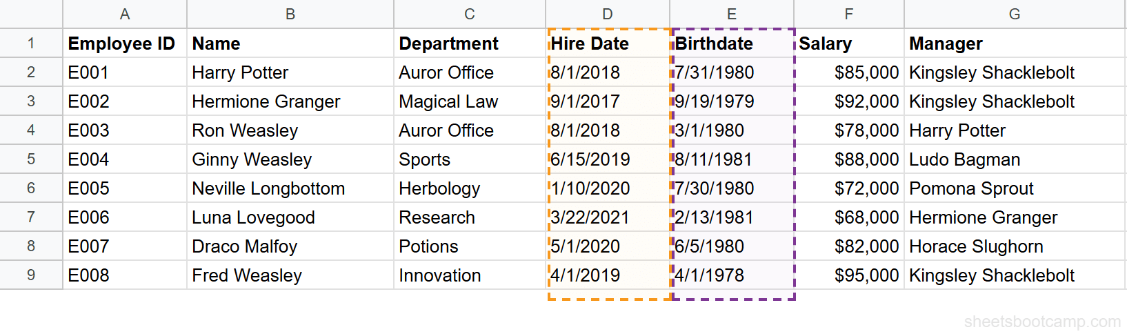
You need a table with date columns to calculate against. The employee database has Hire Date in column D and Birthdate in column E. The data covers 8 employees with hire dates from 2017 through 2021.
2
Calculate years of service with DATEDIF
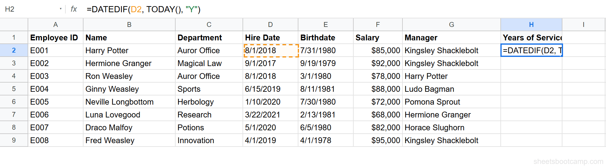
Select cell F2 (or any empty cell) and enter:
Formula
=DATEDIF(D2, TODAY(), "Y") This calculates the number of complete years between Sherlock Holmes’s hire date (8/1/2018) and today. The formula returns 7 (as of July 2026). The "Y" unit counts only full years that have passed.
3
Calculate age from birthdate
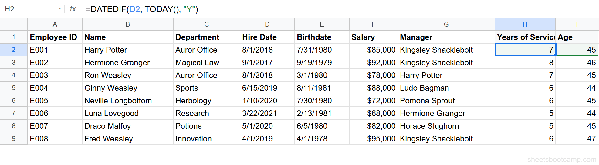
In cell G2, enter:
Formula
=DATEDIF(E2, TODAY(), "Y") Sherlock Holmes’s birthdate is 7/31/1980. The formula returns 45 (as of July 2026). The same DATEDIF pattern works for any “how old” calculation, the only difference is which date column you reference.
Tip
To display tenure as “7 years, 11 months” in a single cell, combine two DATEDIF calls with the ampersand operator: =DATEDIF(D2, TODAY(), "Y") & " years, " & DATEDIF(D2, TODAY(), "YM") & " months". This builds a text string from the numeric results.
4
Make it dynamic with TODAY
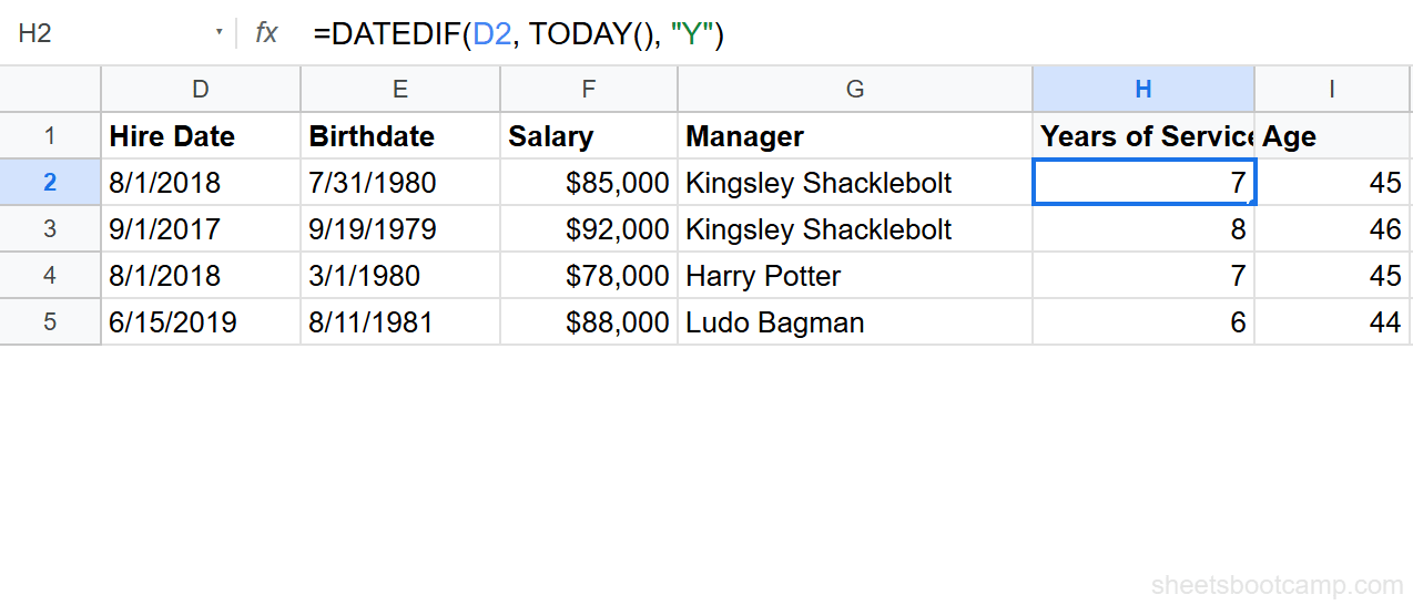
Both formulas already use TODAY() as the end date, so they recalculate automatically each day. Copy the tenure formula from F2 down through F9, and the age formula from G2 down through G9. Each row references its own Hire Date and Birthdate.
5
Review and verify results
Spot-check a few rows:
- Dr. John Watson: Hired 9/1/2017, tenure should be 8 years (as of July 2026)
- Dr. Mortimer: Hired 1/10/2020, tenure should be 6 years
- Sherlock Holmes: Born 7/31/1980, age should be 45 (as of July 2026)
If a value looks wrong, check that the hire date or birthdate cell is formatted as a date, not text. Text values cause DATEDIF to return errors or incorrect results.
Date Function Examples
Example 1: Employee Tenure in Years and Months
A single DATEDIF with "Y" shows complete years, but tenure of “7 years” hides whether someone is 7 years and 1 month or 7 years and 11 months. Use two DATEDIF calls to get both parts.
For Sherlock Holmes (hired 8/1/2018):
Formula
=DATEDIF(D2, TODAY(), "Y") & " yr " & DATEDIF(D2, TODAY(), "YM") & " mo" This returns a text string like “7 yr 11 mo” (the exact months depend on the current date). The "Y" unit counts complete years. The "YM" unit counts the remaining months after those complete years. Together they give a precise tenure display.
Example 2: Next Review Date with EDATE
Company policy says employees get a performance review 6 months after their hire date, then every 6 months after that. Calculate the next review date using EDATE.
For Irene Adler (hired 6/15/2019):
Formula
=EDATE(D5, 6) This returns 12/15/2019, six months after the hire date. To calculate the next upcoming review date from today, you would combine EDATE with a formula that finds the next 6-month interval. A practical approach: =EDATE(D5, CEILING((DATEDIF(D5, TODAY(), "M")), 6)) returns the next review date that falls on or after today.

Example 3: Business Days Between Two Dates with NETWORKDAYS
NETWORKDAYS counts only the working days (Monday-Friday) between two dates, so it is the honest way to measure how much an employee has actually worked. Compare each hire date to today to get business-day tenure:
Formula
=NETWORKDAYS(D2, TODAY()) Sherlock Holmes (hired 8/1/2018) has 2,896 calendar days of tenure but only 2,069 business days once weekends are removed. Mary Morstan (hired 3/22/2021) has 1,932 calendar days and 1,381 business days.

To exclude company holidays from the count, list the holiday dates in a separate range (say, K2:K10) and add it as the third argument: =NETWORKDAYS(D3, D7, K2:K10).
Common Errors and How to Fix Them
Dates Displayed as Numbers
You enter a date formula and the cell shows 46209 instead of 7/6/2026. The formula is correct, the cell format is wrong.
Select the cell (or range), go to Format > Number > Date. The serial number converts to a readable date. This is the most common date “error” in Google Sheets, and it is not a formula problem at all.
#VALUE! Error
A #VALUE! error in a date formula usually means one of the inputs is text that looks like a date but is not recognized by Google Sheets as an actual date.
Test with =ISNUMBER(D2). If it returns FALSE, the cell contains text. Fix it with =DATEVALUE(D2) to convert the text to a proper date, or re-enter the date directly.
This often happens with imported data from CSV files, other spreadsheets, or IMPORTRANGE pulls. The dates look correct visually, but Sheets treats them as text strings.
Tip
When importing dates from external sources, always test one cell with =ISNUMBER() before building formulas on the entire column. Catching text-formatted dates early saves debugging time later.
DATEDIF Returns Wrong Results
DATEDIF requires the start date to come before the end date. If you swap them, the formula returns #NUM!.
Formula
=DATEDIF(TODAY(), D2, "Y") This breaks because TODAY() (2026) is after the hire date (2018). The start date must always be the earlier date:
Formula
=DATEDIF(D2, TODAY(), "Y") Another common issue: the "MD" unit in DATEDIF can return unexpected results in some edge cases. Google’s implementation of "MD" occasionally produces negative numbers or incorrect counts near month boundaries. If you need the day component of a date difference, consider using =DAY(end_date) - DAY(start_date) as a cross-check.
Tips and Best Practices
-
Use TODAY() instead of typing today’s date. Hardcoding “7/6/2026” means the formula stops being accurate tomorrow. TODAY() updates automatically every time the sheet recalculates.
-
Format date columns before entering data. Select the column, go to Format > Number > Date, then start entering dates. This prevents Google Sheets from interpreting date entries as text or numbers.
-
Use DATEDIF for human-readable differences. Subtracting two dates gives you total days, which is useful for calculations but hard to read. DATEDIF with
"Y"and"YM"gives you years and months, which is what people expect to see on reports. -
Store dates as dates, not text. A cell containing the text “January 15, 2024” cannot be used in date math. Use DATEVALUE to convert it, or enter dates in a format Sheets recognizes (1/15/2024, 2024-01-15, or January 15, 2024 typed into a date-formatted cell).
-
Use EDATE instead of adding 30 for “one month.” Adding 30 days is not the same as adding one month. January 31 + 30 days = March 2, not February 28.
=EDATE(A2, 1)correctly handles month lengths and returns February 28 (or 29 in leap years). See adding and subtracting dates for more patterns. -
Combine date functions with conditional formatting for visual alerts. Highlight employees whose tenure exceeds 5 years, flag upcoming review dates, or color-code overdue deadlines. Date functions return numbers, and conditional formatting rules work with number comparisons.
Note
Google Sheets counts dates from December 30, 1899 (day zero), so January 1, 1900 is serial number 2. Excel numbers dates slightly differently (January 1, 1900 is serial 1 there), so serials do not transfer between the two apps as the same dates. For the full reference, see Google’s date function documentation.
Related Google Sheets Tutorials
- TODAY and NOW Functions: Auto-updating current date and time, plus common patterns with DATEDIF
- DATEDIF Function Guide: Calculate differences between dates in years, months, days, and combined units
- EDATE and EOMONTH Functions: Add or subtract months from dates and find month-end dates
- NETWORKDAYS Function: Count business days excluding weekends and holidays
- How to Format Dates: Custom date formats, locale settings, and display options
- YEAR, MONTH, and DAY Functions: Extract parts of a date for grouping and filtering
- DATEVALUE Function: Convert text that looks like a date into a real date
- Add and Subtract Dates: Day, month, and year arithmetic patterns
- WEEKDAY Function: Find which day of the week a date falls on
- Timestamps in Google Sheets: Static vs auto-updating timestamps and keyboard shortcuts
- IF Statements in Google Sheets: Build conditional logic using date comparisons
- QUERY Function Guide: Filter and group data by date ranges using SQL-like syntax
Frequently Asked Questions
How do I calculate the number of days between two dates in Google Sheets?
Use DATEDIF or subtraction. For total days, subtract one date from another: =B2-A2. For years, months, or days separately, use DATEDIF: =DATEDIF(A2, B2, "Y") returns the number of complete years between the two dates.
What is the difference between TODAY and NOW in Google Sheets?
TODAY returns the current date without a time component. NOW returns the current date and time. Use TODAY for date calculations like age or tenure. Use NOW when you need timestamps that include hours and minutes.
Why does my date show as a number in Google Sheets?
Google Sheets stores dates as serial numbers internally, counted from December 30, 1899. If you see a number like 44927 instead of a date, the cell is formatted as a number. Select the cell, go to Format > Number > Date, and the date appears correctly.
How do I add months to a date in Google Sheets?
Use the EDATE function. =EDATE(A2, 6) adds 6 months to the date in A2. To subtract months, use a negative number: =EDATE(A2, -3) goes back 3 months. EDATE keeps the same day of the month when possible.
How do I calculate business days between two dates?
Use NETWORKDAYS. =NETWORKDAYS(A2, B2) counts the weekdays (Monday through Friday) between two dates, excluding weekends. To also exclude holidays, add a range of holiday dates as the third argument: =NETWORKDAYS(A2, B2, holidays).
Can I use DATEDIF in Google Sheets?
Yes, and it autocompletes: typing =DATEDIF brings up the suggestion card, and it is listed under Insert > Function > Date. The syntax is =DATEDIF(start_date, end_date, unit) where unit is "Y" for years, "M" for months, "D" for days, "YM" for months after years, or "MD" for days after months.
How do I convert text to a date in Google Sheets?
Use DATEVALUE. =DATEVALUE("3/15/2024") converts the text string to a date serial number that Google Sheets recognizes as March 15, 2024. Format the result cell as a date to display it properly. DATEVALUE works with most common date text formats.
You've googled this formula before. Probably more than once.
The Bootcamp is a real Google Sheet that grades every formula the moment you press Enter. 193 exercises across 9 modules, the 10% of Sheets that does 90% of the work. One payment of $29.
Get It for $29 Get the Bootcamp for $2930-day refund. Reply to any email and you get your money back.
Not ready to pay? Try Basic Training free →