
VLOOKUP searches the first column of a range for a key and returns a value from another column in the same row. The syntax is =VLOOKUP(search_key, range, index, [is_sorted]), and the last argument should be FALSE for an exact match. For example, =VLOOKUP("SKU-103", A2:D6, 3, FALSE) finds SKU-103 in column A and returns $35.00 from the third column.
beginner 4 min read
VLOOKUP in Google Sheets: Complete Guide
Learn how to use VLOOKUP in Google Sheets with step-by-step examples. Master syntax, fix common errors, and explore alternatives.
SB
Sheets Bootcamp
February 7, 2026 · Updated August 5, 2026
Table of Contents
Quick Answer
VLOOKUP is one of the most useful functions in Google Sheets. It searches for a value in the first column of a range and returns a corresponding value from another column. Whether you’re matching product IDs to prices or employee names to departments, VLOOKUP handles it.
This guide covers everything: syntax, step-by-step examples, common errors, and when to use alternatives like INDEX MATCH.
VLOOKUP Syntax
Watch the four arguments explained (1:21)
Here is the complete VLOOKUP syntax in Google Sheets:
Formula
=VLOOKUP(search_key, range, index, [is_sorted]) | Parameter | Description |
|---|---|
| search_key | The value to search for in the first column of your range |
| range | The range of cells to search (the lookup table) |
| index | The column number in the range to return a value from (starting at 1) |
| is_sorted | FALSE for exact match (recommended), TRUE for approximate match |
Tip
Always use FALSE for the last parameter unless you specifically need approximate matching. Exact matching prevents unexpected results.
Step-by-Step Example
Watch this build, step by step (2:55)
Let’s walk through a real example. You have a product inventory and want to look up prices by product ID.
Sample Data
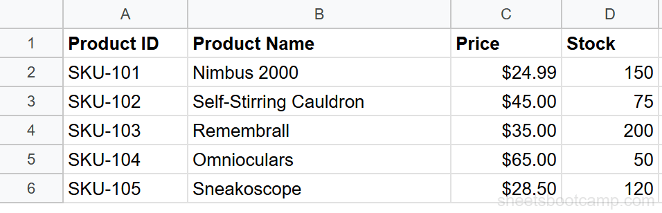
1
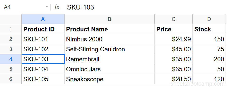
Identify your search value
Decide what you are looking for. In this case, you want to find the price for product ID SKU-103.
2
Write the VLOOKUP formula
Click on an empty cell and enter the formula:
Formula
=VLOOKUP("SKU-103", A2:D6, 3, FALSE) 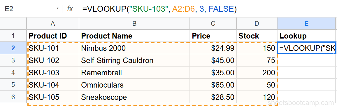
Here is what each part means:
"SKU-103": the product ID to search forA2:D6: the data range (your lookup table)3: return the value from the 3rd column (Price)FALSE: find an exact match
3
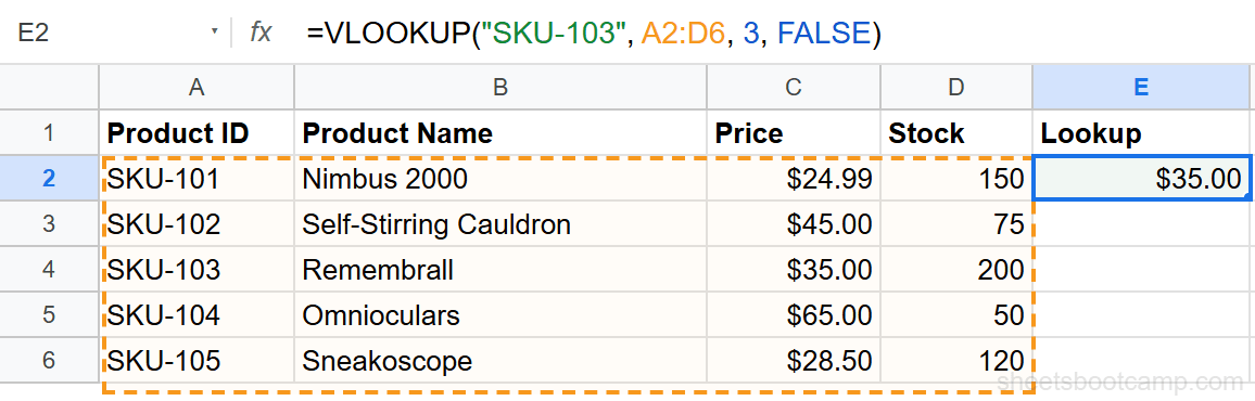
Press Enter to get the result
The formula returns $35.00, which is the price for the Pocket Watch.
4
Make it dynamic with a cell reference
Instead of hardcoding the search value, reference a cell:
Formula
=VLOOKUP(F2, A2:D6, 3, FALSE) Now you can type any product ID in cell F2, and the formula updates automatically.
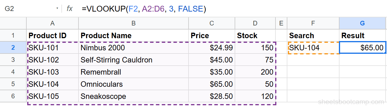
Note
The search key must always be in the first column of your range. If your data is arranged differently, consider using INDEX MATCH instead.
Common VLOOKUP Errors
Watch all three errors get fixed (5:14)
#N/A Error
The #N/A error means VLOOKUP could not find your search key in the lookup range. Common causes:
- Typos in the search key or data
- Extra spaces: use
TRIM()to clean data - Mismatched types: searching for text “123” in a column of numbers
For a full walkthrough of every failure mode and its fix, see fixing VLOOKUP errors.
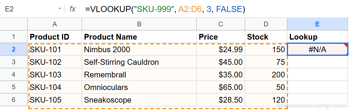
Fix it by wrapping VLOOKUP in IFERROR:
Formula
=IFERROR(VLOOKUP(F2, A2:D6, 3, FALSE), "Not found") #REF! Error
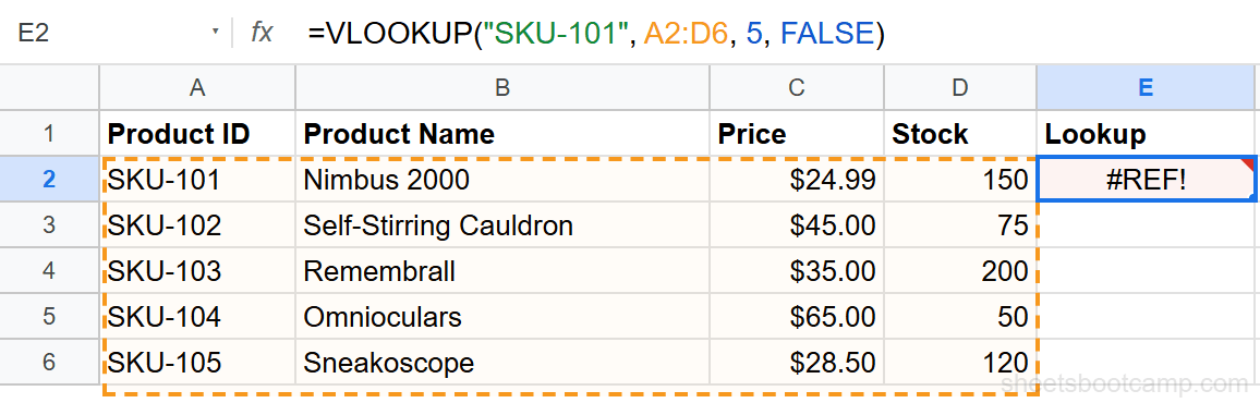
This happens when your index number exceeds the number of columns in the range. If your range has 4 columns, the index must be between 1 and 4.
Warning
Never use an index number larger than the number of columns in your range. A range of A:C has 3 columns, so the maximum index is 3.
#VALUE! Error
The #VALUE! error usually means the index parameter is not a valid number, or the search key is in the wrong format. For example, passing a column name instead of a number triggers it:
Formula
=VLOOKUP("SKU-101", A2:D6, "Price", FALSE) That returns #VALUE! because "Price" is not a column number. Use 3 instead. Note that a quoted number like "3" does not error, because Google Sheets coerces it to a number first.
VLOOKUP with Approximate Match
Watch approximate match in action (6:52)
Setting the last parameter to TRUE enables approximate matching. VLOOKUP finds the largest value less than or equal to your search key.
Important
When using approximate match (TRUE), your first column must be sorted in ascending order. If it is not sorted, VLOOKUP returns incorrect results.
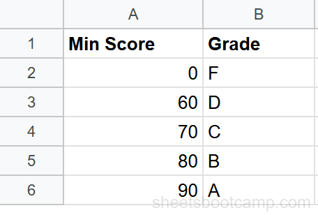
This is useful for grade boundaries, tax brackets, or commission tiers:
Formula
=VLOOKUP(85, A2:B6, 2, TRUE) This returns B because 85 falls between 80 and 89.
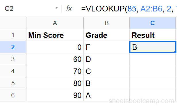
There is more on sorting rules and tier tables in VLOOKUP approximate match.
VLOOKUP vs INDEX MATCH
Watch the three lookups compared (8:02)
| Feature | VLOOKUP | INDEX MATCH |
|---|---|---|
| Lookup direction | Right only | Any direction |
| Column insertions | Breaks formula | Unaffected |
| Speed on large data | Slightly faster | Similar |
| Ease of use | Simpler syntax | More flexible |
| Multiple criteria | Not supported | Supported with arrays |
For straightforward right-lookups, VLOOKUP works well. For anything more complex, INDEX MATCH is the better choice. And if you need to match on more than one condition, there is a workaround in VLOOKUP with multiple criteria.
Best Practices
1. Always use exact match, Set the fourth parameter to FALSE unless you specifically need approximate matching.
2. Lock your range with absolute references, Use $A$2:$D$6 instead of A2:D6 when copying formulas across multiple rows.
3. Wrap in IFERROR, Handle missing values gracefully instead of showing error messages.
4. Keep lookup columns clean, Remove extra spaces, ensure consistent formatting, and avoid mixed data types.
5. Consider alternatives for complex lookups, If you need to look left, match multiple criteria, or handle dynamic column positions, switch to INDEX MATCH or XLOOKUP.
Tip
Google Sheets now supports XLOOKUP, which combines the simplicity of VLOOKUP with the flexibility of INDEX MATCH. Check out our XLOOKUP guide to learn more.
Summary
VLOOKUP is the go-to function for looking up values in Google Sheets. Use it with FALSE for exact matches, wrap it in IFERROR to handle missing data, and switch to INDEX MATCH when you need more flexibility.
Frequently Asked Questions
What does VLOOKUP do in Google Sheets?
VLOOKUP searches for a value in the first column of a range and returns a value from another column in the same row. It stands for 'Vertical Lookup.'
Can VLOOKUP look left in Google Sheets?
No, VLOOKUP can only search the leftmost column and return values from columns to the right. Use INDEX MATCH if you need to look left.
Why does VLOOKUP return #N/A?
The #N/A error means VLOOKUP could not find your search key in the first column of the lookup range. Check for typos, extra spaces, or mismatched data types.
Is VLOOKUP or INDEX MATCH better?
INDEX MATCH is more flexible since it can look in any direction and handles column insertions better. VLOOKUP is simpler to learn and works well for straightforward lookups.
What is the difference between TRUE and FALSE in VLOOKUP?
FALSE finds an exact match, which is what you need in most cases. TRUE finds an approximate match, which is useful for ranges like grade boundaries or tax brackets.
You've googled this formula before. Probably more than once.
The Bootcamp is a real Google Sheet that grades every formula the moment you press Enter. 193 exercises across 9 modules, the 10% of Sheets that does 90% of the work. One payment of $29.
Get It for $29 Get the Bootcamp for $2930-day refund. Reply to any email and you get your money back.
Not ready to pay? Try Basic Training free →