Format Cells Based on Another Cell (Google Sheets)
Learn how to use conditional formatting based on another cell in Google Sheets. Step-by-step custom formula examples with cell references and dynamic thresholds.
Sheets Bootcamp
March 3, 2026
Conditional formatting based on another cell in Google Sheets lets you change one cell’s appearance based on a value in a different cell. Instead of the built-in rules that check a cell against itself, you write a conditional formatting custom formula that references another column or a fixed cell. This unlocks patterns like highlighting revenue when a region matches, or color-coding rows when a status changes.
In This Guide
- How Cell References Work in Conditional Formatting
- Step-by-Step: Format Based on Another Column
- Use a Cell as a Dynamic Threshold
- Practical Examples
- Common Mistakes
- Tips
- Related Google Sheets Tutorials
- FAQ
How Cell References Work in Conditional Formatting
Built-in conditional formatting rules (like “Greater than” or “Text contains”) only compare a cell to a fixed value. To format based on another cell, you need the Custom formula is rule type.
The formula you enter is evaluated relative to the first cell in the “Apply to range” field. If your range starts at F2, the formula runs as though it’s in cell F2 first, then shifts down to F3, F4, and so on.
This is where the dollar sign ($) matters:
| Reference | Behavior | Use Case |
|---|---|---|
$C2 | Column locked to C, row shifts | Check column C for every row |
$C$2 | Both locked | Reference one fixed cell |
C2 | Both shift | Rarely needed in conditional formatting |
The dollar sign controls what stays fixed as the formula moves through each cell in the range. Getting this wrong is the number one reason conditional formatting based on another cell fails.
Step-by-Step: Format Based on Another Column
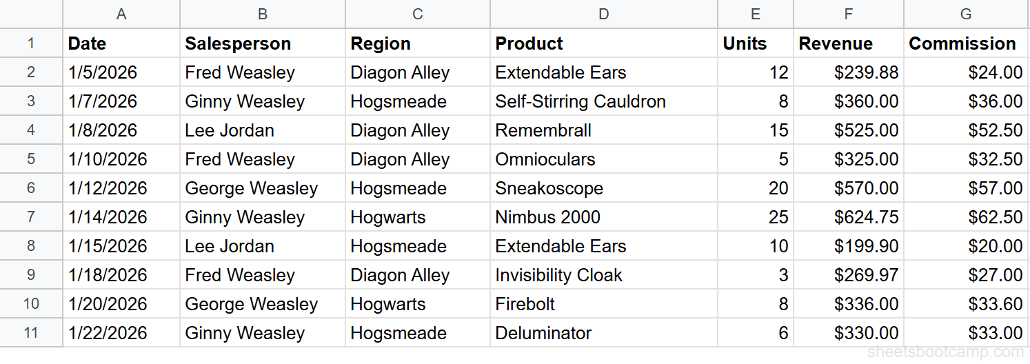
We’ll use a sales records table with 10 transactions. The goal: highlight Revenue cells (column F) green when the Region (column C) is “Hogwarts.”
Sample Data
| A | B | C | D | E | F | G | |
|---|---|---|---|---|---|---|---|
| 1 | Date | Salesperson | Region | Product | Units | Revenue | Commission |
| 2 | 1/5/2026 | Fred Weasley | Diagon Alley | Extendable Ears | 12 | $239.88 | $24.00 |
| 3 | 1/7/2026 | Ginny Weasley | Hogsmeade | Self-Stirring Cauldron | 8 | $360.00 | $36.00 |
| 4 | 1/8/2026 | Lee Jordan | Diagon Alley | Remembrall | 15 | $525.00 | $52.50 |
| 5 | 1/10/2026 | Fred Weasley | Diagon Alley | Omnioculars | 5 | $325.00 | $32.50 |
| 6 | 1/12/2026 | George Weasley | Hogsmeade | Sneakoscope | 20 | $570.00 | $57.00 |
| 7 | 1/14/2026 | Ginny Weasley | Hogwarts | Nimbus 2000 | 25 | $624.75 | $62.50 |
| 8 | 1/15/2026 | Lee Jordan | Hogsmeade | Extendable Ears | 10 | $199.90 | $20.00 |
| 9 | 1/18/2026 | Fred Weasley | Diagon Alley | Invisibility Cloak | 3 | $269.97 | $27.00 |
| 10 | 1/20/2026 | George Weasley | Hogwarts | Firebolt | 8 | $336.00 | $33.60 |
| 11 | 1/22/2026 | Ginny Weasley | Hogsmeade | Deluminator | 6 | $330.00 | $33.00 |
Select the range to format
Highlight cells F2 through F11 — the Revenue column. This is the range that will receive the formatting, even though the condition checks a different column.
Open conditional formatting and choose Custom formula is
Go to Format > Conditional formatting. In the Format rules dropdown, select Custom formula is and enter:
=$C2="Hogwarts"The $C locks the column to C (Region). The 2 is relative and shifts for each row. When the formula evaluates row 7, it checks $C7="Hogwarts" — which is TRUE for Ginny Weasley’s Nimbus 2000 transaction.
Choose a fill color and apply
Click the paint bucket icon and select green. Click Done.
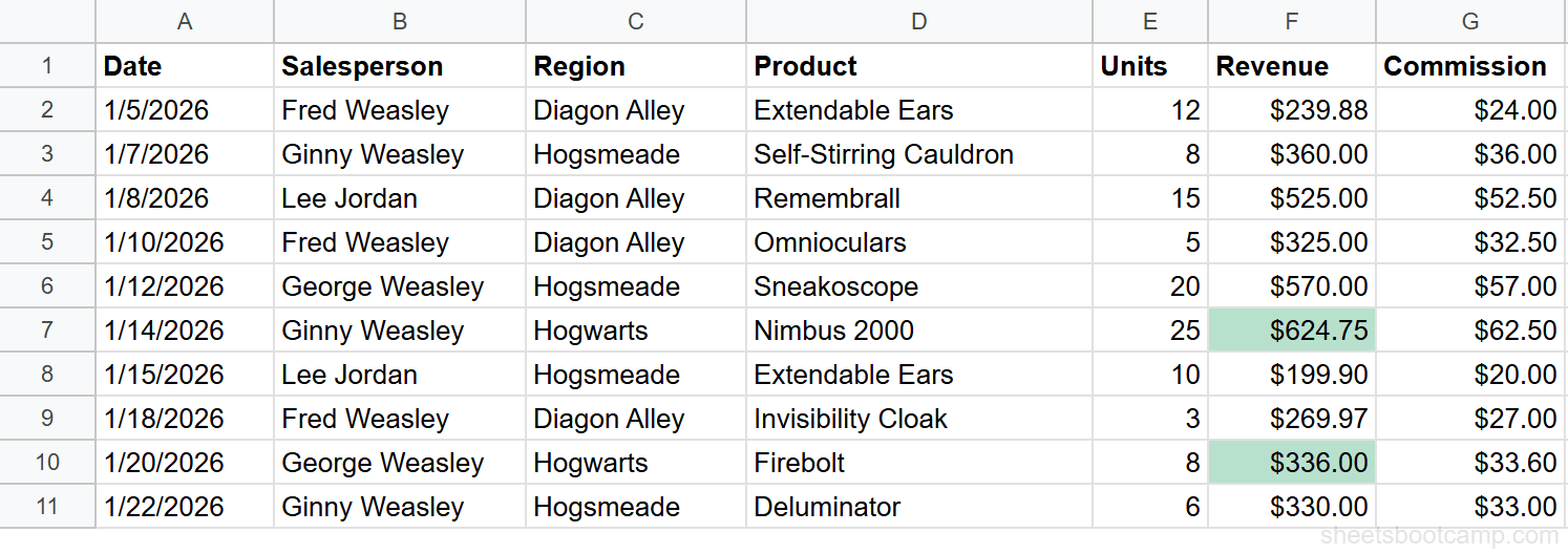
Review the result
Two Revenue cells are highlighted green: $624.75 (row 7, Ginny Weasley at Hogwarts) and $336.00 (row 10, George Weasley at Hogwarts). Every other Revenue cell stays white because its corresponding Region cell is not “Hogwarts.”
Use a Cell as a Dynamic Threshold
Instead of hardcoding a value into the formula, reference a cell that holds the threshold. This way, you change one cell and the formatting updates across the entire range.
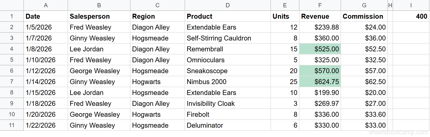
Suppose cell I1 contains 400. Apply this rule to F2:F11:
=F2>$I$1The $I$1 is fully locked — every cell in the range compares its Revenue value against the same threshold in I1. Three cells are highlighted: $525.00, $570.00, and $624.75 (all above 400).
Change I1 to 300 and the formatting instantly updates to include $360.00, $325.00, $336.00, and $330.00 as well.
A dynamic threshold is useful when you share a spreadsheet with others. They can adjust the threshold without editing the conditional formatting rule.
Practical Examples
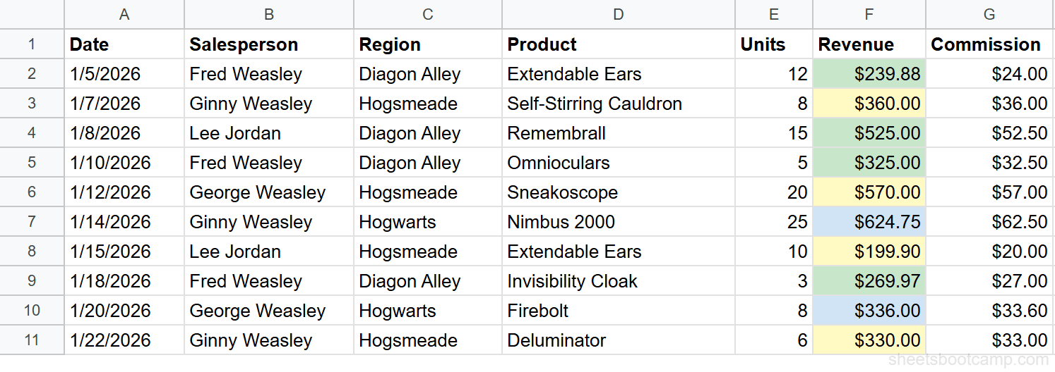
Example 1: Color-Code Revenue by Region
Apply three separate rules to F2:F11, in this order:
=$C2="Hogwarts"→ Blue fill=$C2="Hogsmeade"→ Yellow fill=$C2="Diagon Alley"→ Green fill
Each rule checks the Region column for the current row and applies a different color to the Revenue cell. The result: a color-coded Revenue column where you can see which region each transaction belongs to at a glance.
Example 2: Highlight When Units Exceed a Threshold
Format the Product column (D2:D11) to highlight product names when the Units column (E) exceeds 15:
=$E2>15Two Product cells are highlighted: Sneakoscope (20 units in row 6) and Nimbus 2000 (25 units in row 7). No other row exceeds 15 units.
Example 3: Format Based on a Text Status
If you add a Status column (H) with values like “Complete” or “Pending,” you can highlight the Salesperson column based on that status:
=$H2="Complete"Applied to B2:B11, this highlights any salesperson name where the corresponding Status cell says “Complete.” The formula checks column H for every row, and the formatting applies to column B.
Common Mistakes
Forgetting the dollar sign on the column reference
If you write =C2="Hogwarts" instead of =$C2="Hogwarts", the column reference shifts as the formula moves across the range. For cell F2, the formula checks C2 (correct). But for cell G2, it checks D2 (wrong). Locking the column with $C ensures the formula always checks the Region column.
Applying the rule to the wrong range
If you select A2:G11 but only want the Revenue column formatted, the formatting appears in every column. Select only the cells you want to change color — in this case, F2:F11. The formula can reference any cell on the sheet, but the “Apply to range” controls which cells actually get formatted.
Text comparison is case-sensitive
=$C2="hogwarts" does not match “Hogwarts” because the comparison is case-sensitive. Either match the exact casing or use LOWER: =LOWER($C2)="hogwarts".
If your formula works when you test it in a regular cell but does nothing in conditional formatting, check that you selected “Custom formula is” from the dropdown. Other rule types ignore formula syntax and treat it as a literal text comparison.
Tips
Test formulas in a cell first. Enter =$C2="Hogwarts" in an empty cell next to your data to verify it returns TRUE and FALSE for the correct rows. Then paste it into the conditional formatting rule.
Name your threshold cells. If you use a dynamic threshold in I1, add a label in H1 like “Threshold” so collaborators know what the cell controls.
Combine with data validation. Use a data validation dropdown in your threshold cell to restrict inputs to valid values. This prevents someone from accidentally entering text where a number is expected.
Related Google Sheets Tutorials
- Conditional Formatting: Complete Guide — covers all rule types, color scales, and managing multiple rules
- Conditional Formatting Entire Row — apply formatting across all columns based on one cell’s value
- Custom Formula in Conditional Formatting — write advanced rules with any formula that returns TRUE or FALSE
- IF Function: Complete Guide — use IF for logical tests in formulas, a natural companion to conditional formatting rules
Frequently Asked Questions
How do I apply conditional formatting based on another cell value?
Use a Custom formula is rule. Select the range to format, choose “Custom formula is” from the dropdown, and enter a formula that references the other cell. For example, =$C2="Hogwarts" applied to F2:F11 highlights Revenue cells where the Region column says “Hogwarts.” The $C locks the column reference so the formula always checks column C.
Can I reference a cell in conditional formatting Google Sheets?
Yes. Choose “Custom formula is” as the rule type and write a formula that points to any cell. Use a dollar sign to lock the column or row reference as needed. The formula evaluates relative to the first cell in the “Apply to range” field, and the references shift row by row.
How do I use a cell reference as a threshold in conditional formatting?
Enter a formula like =F2>$I$1 where I1 contains your threshold value. The absolute reference $I$1 stays fixed so every cell in the range compares against the same threshold. Change the value in I1 and the formatting updates instantly without editing the rule.
Why is my conditional formatting based on another cell not working?
The most common cause is a missing or misplaced dollar sign. If your formula references a column that should stay fixed, lock it with a dollar sign like $C2. Also verify you selected “Custom formula is” from the dropdown — other rule types treat formula syntax as literal text. Finally, check that the text casing matches exactly, since comparisons are case-sensitive.