Conditional Formatting with Dates in Google Sheets
Learn how to use conditional formatting with dates in Google Sheets. Highlight overdue dates, upcoming deadlines, and past dates with custom formula rules.
Sheets Bootcamp
June 2, 2026
Conditional formatting with dates in Google Sheets highlights cells based on when something is due, when it happened, or how close it is to today. Combined with the TODAY() function, date rules update automatically every day. You set the rule once, and overdue tasks turn red, upcoming deadlines turn yellow, and completed items stay green without you touching a thing.
In This Guide
- How Date Formatting Rules Work
- Step-by-Step: Highlight Overdue Dates
- Highlight Dates in the Next 7 Days
- Highlight Dates Older Than 30 Days
- Color-Code by Date Range (Multi-Rule)
- Format an Entire Row Based on a Date
- Common Mistakes
- Tips
- Related Google Sheets Tutorials
- FAQ
How Date Formatting Rules Work
Google Sheets stores dates as numbers. January 1, 1900 is 1, January 2 is 2, and so on. When you write a custom formula like =C2<TODAY(), Sheets compares the numeric value of the date in C2 to today’s numeric value. If C2 is smaller (earlier), the condition is true and the formatting applies.
This means any date comparison you can write in a formula also works in conditional formatting:
| Formula | What It Highlights |
|---|---|
=C2<TODAY() | Dates in the past |
=C2>TODAY() | Dates in the future |
=C2=TODAY() | Today’s date only |
=C2<TODAY()-30 | Dates more than 30 days ago |
=AND(C2>=TODAY(), C2<=TODAY()+7) | Dates within the next 7 days |
The TODAY function recalculates every time the spreadsheet opens or recalculates. Your formatting rules stay current without any manual effort.
Date conditional formatting only works on actual date values, not text that looks like a date. If your dates were typed as plain text or imported as strings, Sheets won’t compare them correctly. Select the column and check Format > Number. If it says Plain text, change it to Date first.
Step-by-Step: Highlight Overdue Dates
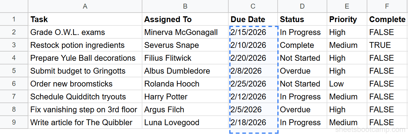
We’ll use the task tracker to highlight any due date that has already passed.
Step 1: Select the Date Column and Open Conditional Formatting
Highlight the cells containing due dates. In the task tracker, select C2:C12 (the Due Date column, not the header).
Go to Format > Conditional formatting.
Step 2: Choose Custom Formula Is and Enter a Date Formula
In the Conditional format rules panel, select Custom formula is from the dropdown.
Enter the formula:
=C2<TODAY()This checks whether the date in C2 is before today. Sheets evaluates the formula for each cell in the range, shifting the row reference automatically. C2 becomes C3, then C4, and so on.
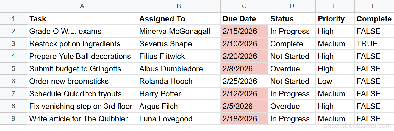
Step 3: Set the Formatting Style and Click Done
Choose a red fill color (light red works well for overdue items). Click Done.
Every date before today turns red. As days pass, more dates will turn red automatically because TODAY() updates.
Combine this with a status column check to avoid highlighting completed tasks. Use =AND(C2<TODAY(), $D2<>"Complete") so only overdue items that are still open get the red fill.
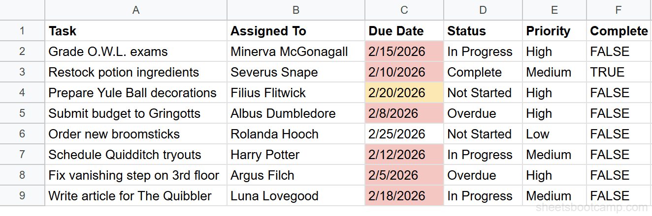
Highlight Dates in the Next 7 Days
Overdue items need attention, but so do items that are coming up soon. A “due this week” rule catches deadlines before they pass.
Select C2:C12 and add a new conditional formatting rule with this formula:
=AND(C2>=TODAY(), C2<=TODAY()+7)Set a yellow or orange fill color. This highlights any date from today through seven days out.
The AND function requires both conditions to be true: the date is on or after today, and the date is within the next 7 days. Change the 7 to any number. Use 3 for “due in the next three days” or 14 for a two-week window.
When you have multiple rules on the same range, Google Sheets applies them in order from top to bottom. If a date is both overdue and within 7 days of today (which can not happen simultaneously), the first matching rule wins. Drag rules to reorder them in the Conditional format rules panel.
Highlight Dates Older Than 30 Days
For tracking stale items, invoices past due, or anything that should have been handled long ago:
=C2<TODAY()-30This highlights any date more than 30 days in the past. Use a dark red or bold red fill to distinguish “very overdue” from “recently overdue.”
You can use the same pattern for any time window:
| Formula | Meaning |
|---|---|
=C2<TODAY()-7 | More than a week ago |
=C2<TODAY()-30 | More than a month ago |
=C2<TODAY()-90 | More than three months ago |
=C2<TODAY()-365 | More than a year ago |
Color-Code by Date Range (Multi-Rule)
Stack multiple rules on the same range to build a traffic-light system:
| Rule (in order) | Formula | Fill Color | Meaning |
|---|---|---|---|
| 1 | =C2<TODAY() | Red | Overdue |
| 2 | =AND(C2>=TODAY(), C2<=TODAY()+3) | Orange | Due within 3 days |
| 3 | =AND(C2>TODAY()+3, C2<=TODAY()+7) | Yellow | Due within a week |
| 4 | =C2>TODAY()+7 | Green | More than a week out |
Apply these four rules to C2:C12 in this order. The first rule that matches gets applied. Since rules are evaluated top to bottom, put the most urgent condition first.
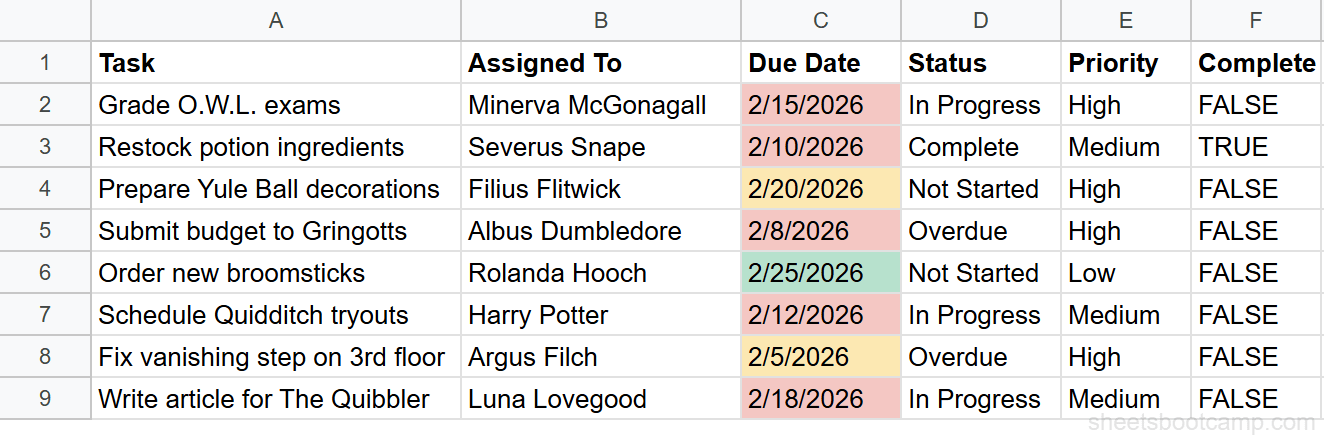
The result is a due date column that tells you at a glance what needs attention right now (red), what’s coming soon (orange/yellow), and what can wait (green).
Format an Entire Row Based on a Date
Highlighting a single date cell is useful, but highlighting the entire row for overdue tasks makes the pattern even clearer. To do this, expand the range and lock the column reference.
Select A2:F12 (the full data range, not the headers). Add a Custom formula is rule:
=$C2<TODAY()The dollar sign on $C locks the column reference. As Sheets evaluates each cell in the row, it always checks column C for the date, but the row shifts as expected. Every cell in a row with an overdue date gets the red fill.
This works because conditional formatting evaluates the formula relative to each cell in the “Apply to” range. For cell A2, the formula becomes =$C2<TODAY(). For cell B2, it’s still =$C2<TODAY() because the column is locked. For cell A3, it shifts to =$C3<TODAY().
For the full walkthrough on row-based rules, see the entire row conditional formatting guide.
Common Mistakes
Dates Stored as Text
The most common reason date rules fail. If dates were imported from a CSV or typed with an unrecognized format, Sheets may store them as text strings instead of date values. The formula =C2<TODAY() compares a number to a text string and returns FALSE.
Fix: Select the column, go to Format > Number > Date. If that doesn’t work, the values are embedded as text. Use =DATEVALUE(C2) in a helper column to convert them, then apply formatting to the helper column.
Wrong Row Reference in the Formula
If you apply the rule to C2:C12 but write =C1<TODAY(), the formula is off by one row. Cell C2 evaluates =C1<TODAY() (the header row), C3 evaluates =C2<TODAY(), and the entire rule is shifted.
Fix: The formula should reference the first row in your “Apply to” range. If the range starts at C2, the formula starts with C2.
Missing Dollar Sign for Row Rules
When formatting an entire row based on a date column, =C2<TODAY() shifts both the column and the row. By the time the formula reaches column D, it’s checking D2 instead of C2.
Fix: Lock the column with a dollar sign: =$C2<TODAY(). The row still shifts, but the column stays on C.
Tips
-
Use TODAY() for dynamic rules, fixed dates for static ones. If the deadline is always March 15, use
=C2<DATE(2026,3,15)instead of TODAY(). This prevents the rule from changing over time. -
Combine date rules with IF with AND/OR logic. Formulas like
=AND($C2<TODAY(), $D2<>"Complete")filter out rows that are overdue but already handled. -
Check rule order when stacking. Google Sheets applies the first matching rule. If your “overdue” rule is below your “due soon” rule, an overdue date might get the wrong color. Drag the most important rule to the top.
-
Test your formula in a regular cell first. Enter
=C2<TODAY()in an empty cell. If it returns TRUE for dates you expect to highlight, the formula is correct. Then move it to the conditional formatting rule. -
Remember that TODAY() recalculates. Rules using TODAY() change every day. A date that was “due in 3 days” yesterday is “due in 2 days” today. This is usually what you want, but be aware of it when reviewing historical snapshots.
Related Google Sheets Tutorials
- Conditional Formatting in Google Sheets - Full guide to all conditional formatting rule types
- Custom Formula in Conditional Formatting - Write formula-based rules beyond the built-in presets
- TODAY and NOW Functions - How the TODAY function works and when to use NOW instead
- Conditional Formatting Entire Row - Highlight full rows based on a single cell’s value
- Google Sheets Date Functions - Complete reference for all date functions
Frequently Asked Questions
How do I highlight overdue dates in Google Sheets?
Select the date column, go to Format > Conditional formatting, choose Custom formula is, and enter =C2<TODAY(). Set a red fill color and click Done. Any date before today turns red automatically. The rule updates every day because TODAY() recalculates.
Can I use TODAY() in conditional formatting?
Yes. TODAY() works inside Custom formula is rules. It returns the current date and recalculates daily, so your formatting always reflects the current date without manual updates. Use it to highlight past dates, upcoming deadlines, or dates within a specific range.
How do I highlight dates within the next 7 days in Google Sheets?
Use the Custom formula is rule =AND(C2>=TODAY(), C2<=TODAY()+7). This highlights dates from today through seven days from now. Adjust the number to change the window. For example, TODAY()+30 catches anything in the next month.
Why is my date conditional formatting not working?
The most common cause is that your dates are stored as text, not actual date values. Check by selecting a cell and looking at the format. If it shows Plain text, change it to Date using Format > Number > Date. Also make sure your formula references the correct first row of your apply-to range.
How do I format an entire row based on a date in one column?
Select the full row range (like A2:F12) and use a Custom formula is rule with a locked column reference like =$C2<TODAY(). The dollar sign on C locks the column, so every cell in the row checks the same date column. All cells in rows with overdue dates get the formatting.