Conditional Formatting Entire Row in Google Sheets
Learn how to highlight an entire row with conditional formatting in Google Sheets. Custom formula examples for row-based formatting by cell value.
Sheets Bootcamp
March 4, 2026
Conditional formatting for an entire row in Google Sheets highlights every column in a row when one cell matches a condition. The built-in rule types only format the cells they evaluate, so you need a conditional formatting custom formula with a locked column reference. This guide covers the technique step by step, with three practical examples using real sales data.
In This Guide
- Why Entire-Row Formatting Needs a Custom Formula
- Step-by-Step: Highlight Rows by Region
- Practical Examples
- How the Dollar Sign Works
- Common Mistakes
- Tips
- Related Google Sheets Tutorials
- FAQ
Why Entire-Row Formatting Needs a Custom Formula
If you select column C and add a rule for “Text is exactly Hogwarts,” only column C cells turn color. The other columns in those rows stay white. That is because built-in rules format only the cells in the “Apply to range.”
To color the entire row, you need two things:
- Apply to range covers all columns — select A2:G11, not C2:C11.
- A custom formula with a locked column —
=$C2="Hogwarts"always checks column C, regardless of which column the formula is evaluating.
When Sheets evaluates cell A2, it runs =$C2="Hogwarts". When it evaluates B2, it still runs =$C2="Hogwarts". The $ on the column means it never shifts away from C. But the row number is relative, so for row 3 it checks =$C3, for row 4 it checks =$C4, and so on.
The “Apply to range” controls which cells get colored. The formula controls which rows match. Both must be correct for entire-row formatting to work.
Step-by-Step: Highlight Rows by Region
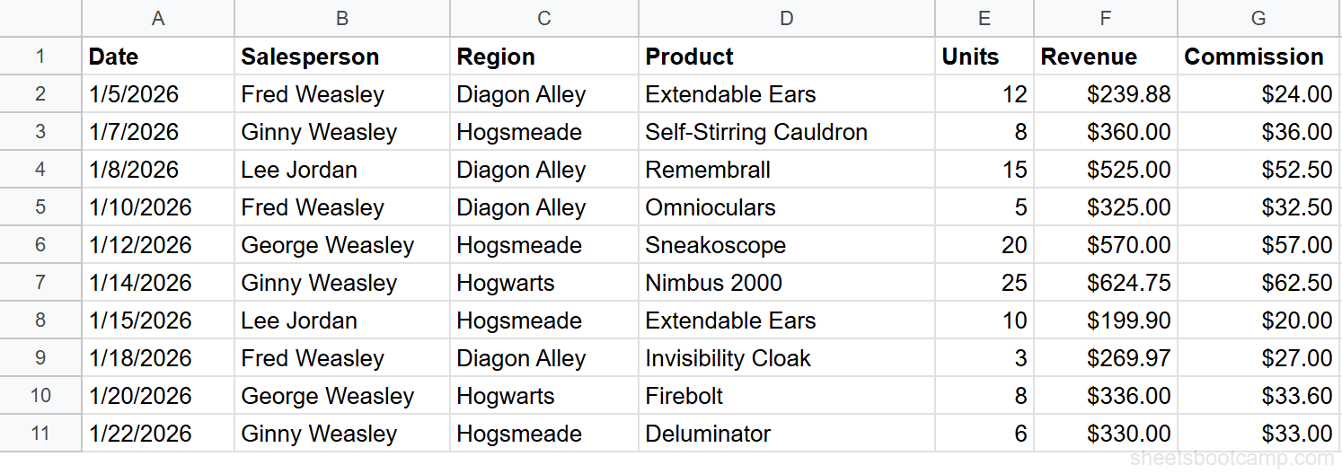
We’ll use a sales records table with 10 transactions. The goal: highlight every column in rows where the Region is “Hogwarts.”
Sample Data
| A | B | C | D | E | F | G | |
|---|---|---|---|---|---|---|---|
| 1 | Date | Salesperson | Region | Product | Units | Revenue | Commission |
| 2 | 1/5/2026 | Fred Weasley | Diagon Alley | Extendable Ears | 12 | $239.88 | $24.00 |
| 3 | 1/7/2026 | Ginny Weasley | Hogsmeade | Self-Stirring Cauldron | 8 | $360.00 | $36.00 |
| 4 | 1/8/2026 | Lee Jordan | Diagon Alley | Remembrall | 15 | $525.00 | $52.50 |
| 5 | 1/10/2026 | Fred Weasley | Diagon Alley | Omnioculars | 5 | $325.00 | $32.50 |
| 6 | 1/12/2026 | George Weasley | Hogsmeade | Sneakoscope | 20 | $570.00 | $57.00 |
| 7 | 1/14/2026 | Ginny Weasley | Hogwarts | Nimbus 2000 | 25 | $624.75 | $62.50 |
| 8 | 1/15/2026 | Lee Jordan | Hogsmeade | Extendable Ears | 10 | $199.90 | $20.00 |
| 9 | 1/18/2026 | Fred Weasley | Diagon Alley | Invisibility Cloak | 3 | $269.97 | $27.00 |
| 10 | 1/20/2026 | George Weasley | Hogwarts | Firebolt | 8 | $336.00 | $33.60 |
| 11 | 1/22/2026 | Ginny Weasley | Hogsmeade | Deluminator | 6 | $330.00 | $33.00 |
Select the full row range
Highlight cells A2 through G11 — the entire data area excluding the header. This is the range that will receive formatting. Selecting all seven columns is what makes the entire row light up, not a single column.
Open conditional formatting
Go to Format > Conditional formatting. The “Apply to range” field should show A2:G11. If it shows a smaller range, type A2:G11 manually.
Enter the custom formula
In the Format rules dropdown, select Custom formula is and enter:
=$C2="Hogwarts"The $C locks to the Region column. The row number 2 is relative — it adjusts for each row in the range.
Set the fill color and apply
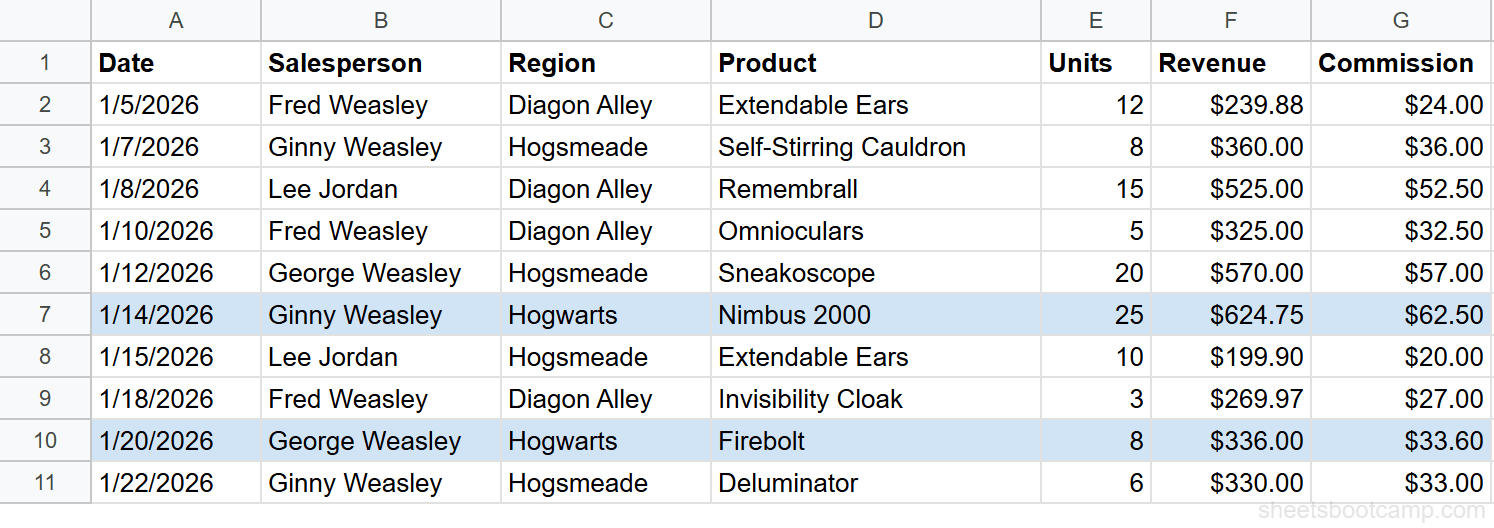
Choose a light blue fill color and click Done.
Two entire rows are highlighted: row 7 (Ginny Weasley, Hogwarts, Nimbus 2000, $624.75) and row 10 (George Weasley, Hogwarts, Firebolt, $336.00). Every column from A to G is colored because the “Apply to range” covers all seven columns.
Practical Examples
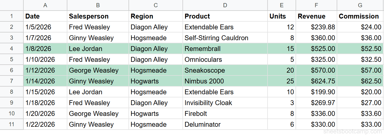
Example 1: Highlight Rows Where Revenue Exceeds $500
Apply to A2:G11 with:
=$F2>500The $F locks to the Revenue column. Three rows are highlighted:
- Row 4: Lee Jordan, Remembrall, $525.00
- Row 6: George Weasley, Sneakoscope, $570.00
- Row 7: Ginny Weasley, Nimbus 2000, $624.75
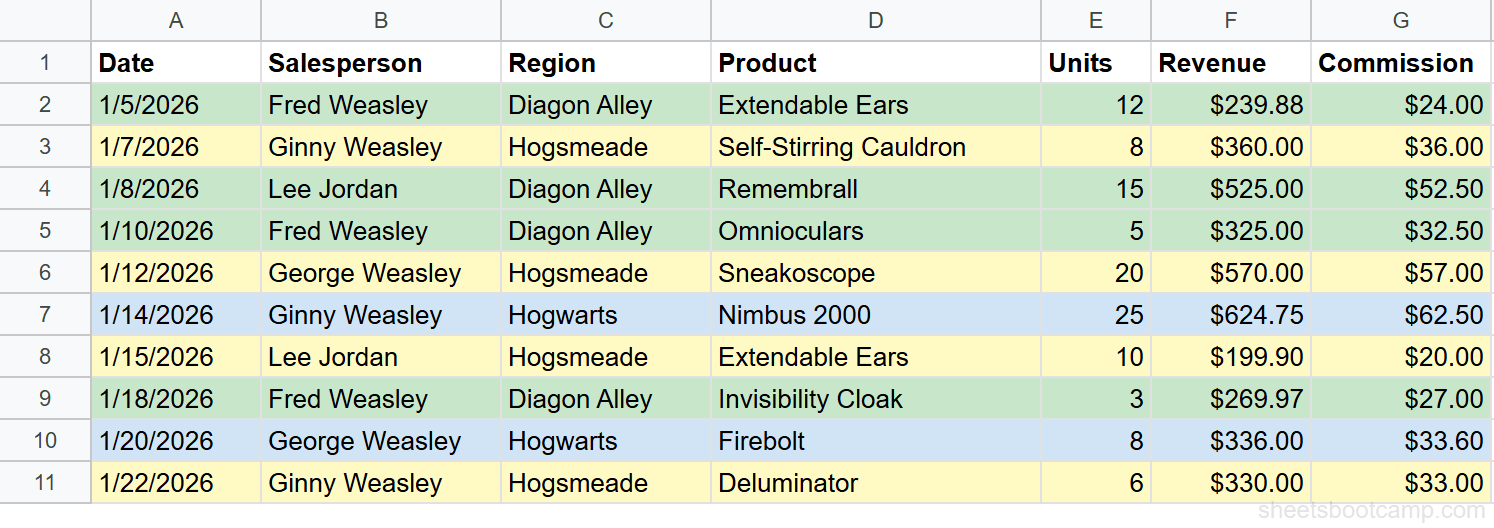
Example 2: Multiple Row Colors by Region
Stack three rules on A2:G11 to color-code by region:
=$C2="Hogwarts"→ Light blue fill=$C2="Hogsmeade"→ Light yellow fill=$C2="Diagon Alley"→ Light green fill
Each rule checks the Region column and applies a different color to the entire row. The result is a spreadsheet where you can identify each transaction’s region at a glance.
When stacking rules, add them from most specific to least specific. Sheets evaluates rules top to bottom and the first match wins. If two rules could match the same row, the rule higher in the list determines the color.
Example 3: Highlight Rows with Above-Average Revenue
Apply to A2:G11 with:
=$F2>AVERAGE($F$2:$F$11)The AVERAGE of the 10 revenue values is $378.05. Three rows exceed that average: Lee Jordan ($525.00), George Weasley ($570.00), and Ginny Weasley ($624.75). The $F$2:$F$11 range is fully locked so the average calculation stays fixed for every cell.
How the Dollar Sign Works
The dollar sign is the key to entire-row formatting. Here is what each reference style does in a conditional formatting formula applied to A2:G11:
| Reference | Column | Row | What Happens |
|---|---|---|---|
=$C2 | Locked to C | Shifts per row | Always checks Region column — correct for row formatting |
$C$2 | Locked to C | Locked to row 2 | Always checks C2 — same value for every row |
=C2 | Shifts per column | Shifts per row | Checks C for column A, D for column B, E for column C — wrong |
=C$2 | Shifts per column | Locked to row 2 | Checks different columns in row 2 only — rarely useful |
For entire-row formatting, always lock the column with $ and leave the row relative. This ensures the formula checks the same column for every cell in the row, while moving down one row at a time.
If you forget the $ on the column, the formula shifts right as it evaluates each column. Cell A2 checks C2 (Region), but cell D2 checks F2 (Revenue), and cell E2 checks G2 (Commission). The formatting becomes unpredictable.
Common Mistakes
Selecting only one column instead of the full range
If “Apply to range” is C2:C11, only column C gets colored even if the formula is correct. Change it to A2:G11 to cover all columns.
Forgetting the $ on the column reference
=C2="Hogwarts" shifts the column for each cell in the row. For cell A2 the formula checks C2 (correct), but for cell B2 it checks D2 (Product — wrong). Always write =$C2.
Rule order conflicts with multiple colors
If you add “Hogwarts = blue” below “Hogsmeade = yellow” but a row somehow matches both, the higher rule wins. Drag rules in the conditional formatting panel to reorder them. Put the most important color at the top.
Formatting applies to the header row
If your range starts at A1 instead of A2, the header row gets colored too. Always start the “Apply to range” at the first data row, not the header.
Tips
Select the range before opening the panel. Highlight A2:G11 first, then open Format > Conditional formatting. This pre-fills the “Apply to range” field and saves a step.
Use alternating colors for readability. Combine entire-row conditional formatting with Sheets’ built-in alternating colors (Format > Alternating colors) for rows that do not match any rule. This keeps the spreadsheet easy to scan.
Add a legend. If you use multiple colors for different categories, add a small key at the top or side of the sheet explaining what each color means. This helps collaborators who did not set up the rules.
Related Google Sheets Tutorials
- Conditional Formatting: Complete Guide — all rule types, color scales, and multiple rule management
- Format Based on Another Cell — highlight one column based on a value in a different column
- Custom Formula in Conditional Formatting — write advanced rules with any formula that returns TRUE or FALSE
- IF Function: Complete Guide — use IF for logical tests in formulas, a companion to conditional formatting logic
Frequently Asked Questions
How do I highlight an entire row based on a cell value in Google Sheets?
Select the full data range (like A2:G11), choose “Custom formula is,” and enter a formula with a locked column reference. For example, =$C2="Hogwarts" checks the Region column and highlights every column in rows where it matches. The $ on the column is what makes the formula check the same column for every cell in the row.
Why does my conditional formatting only color one column instead of the whole row?
Your “Apply to range” only covers one column. To highlight the entire row, the range must span all columns — for example, A2:G11 instead of C2:C11. The formula determines which rows match. The range determines which cells get colored.
Can I apply different colors to different rows with conditional formatting?
Yes. Create multiple rules on the same range (A2:G11) with different formulas and colors. For example, =$C2="Hogwarts" with blue and =$C2="Hogsmeade" with yellow. Rules are evaluated top to bottom, and the first match wins. Drag rules to reorder them in the conditional formatting panel.
What does the dollar sign do in conditional formatting formulas?
The dollar sign locks a reference so it does not shift. In =$C2, the $ locks the column to C while the row number shifts for each row. This ensures every cell in the row checks the same column. Without it, the column reference shifts across columns and checks the wrong data.