Data Validation with Custom Formula in Google Sheets
Learn how to use custom formula data validation in Google Sheets. Restrict cell input with any formula that returns TRUE or FALSE. Step-by-step examples.
Sheets Bootcamp
June 3, 2026
Custom formula data validation in Google Sheets lets you write any formula that returns TRUE or FALSE to control what users can enter. The built-in criteria (dropdown, number, date) cover common cases, but custom formulas handle everything else: character limits, pattern matching, duplicate prevention, cross-column checks, and multi-condition rules. If you can express the rule as a formula, you can enforce it as validation.
In This Guide
- How Custom Formula Validation Works
- Step-by-Step: Limit Text Length
- Prevent Duplicate Entries
- Enforce a Text Pattern with REGEXMATCH
- Validate Based on Another Column
- Combine Multiple Conditions with AND/OR
- Common Mistakes
- Tips
- Related Google Sheets Tutorials
- FAQ
How Custom Formula Validation Works
When you select Custom formula is in the Data validation panel, Google Sheets evaluates your formula every time someone enters a value in the validated range. The formula must return TRUE (allow) or FALSE (reject).
The formula you enter references the first cell in your apply-to range. If your range is A2:A12, write the formula as if it applies to A2. Sheets automatically shifts the row reference for each cell in the range, just like a formula copied down a column.
| Your Formula | Cell A2 Evaluates | Cell A3 Evaluates | Cell A4 Evaluates |
|---|---|---|---|
=LEN(A2)<=40 | =LEN(A2)<=40 | =LEN(A3)<=40 | =LEN(A4)<=40 |
=A2>0 | =A2>0 | =A3>0 | =A4>0 |
The formula must reference the first row of the apply-to range. If your range starts at A2, use A2 in the formula. If it starts at A5, use A5. Getting this wrong shifts every row’s check by the offset.
Reject Input vs Show Warning
After entering the formula, you choose how Sheets handles invalid data:
- Reject input: Blocks the entry entirely. The cell reverts to its previous value and shows an error popup.
- Show warning: Allows the entry but marks the cell with an orange warning triangle. The data stays, but the user sees a flag.
For rules that enforce data integrity (no duplicates, required formats), use Reject input. For soft guidelines (recommended length, preferred format), Show warning gives users flexibility.
Step-by-Step: Limit Text Length
We’ll use the task tracker to limit task names in column A to 40 characters.
Step 1: Select the Cells and Open Data Validation
Highlight A2:A12 in the task tracker — the cells in the Task column where users enter task names.
Go to Data > Data validation.
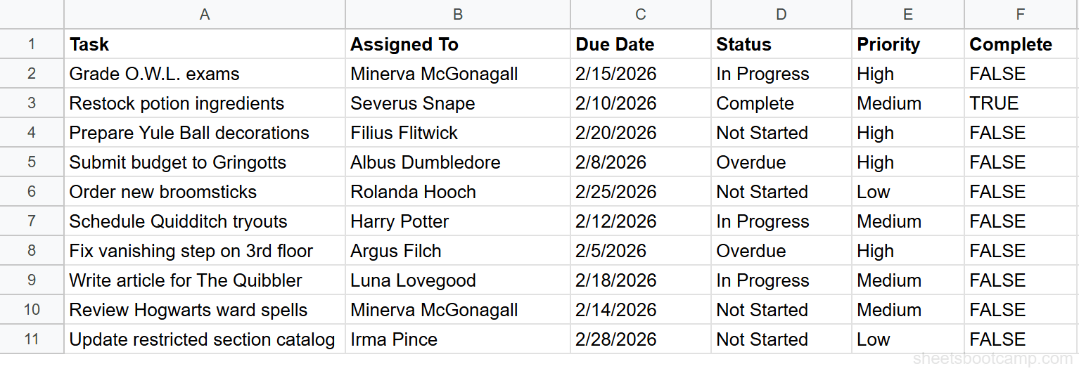
Step 2: Choose Custom Formula Is and Enter Your Formula
In the Data validation panel, click Add rule. Under Criteria, select Custom formula is from the dropdown.
Enter the formula:
=LEN(A2)<=40This checks the character count of whatever is typed in A2. If it’s 40 or fewer, the formula returns TRUE and the input is accepted. If it’s 41 or more, the formula returns FALSE and the input is rejected.
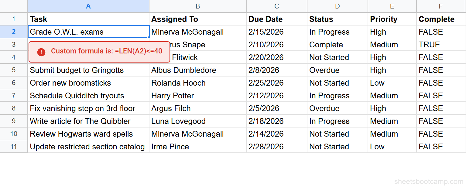
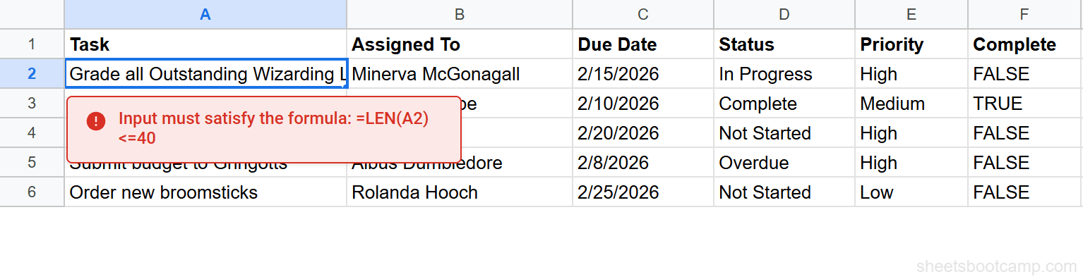
Step 3: Set Rejection Behavior and Click Done
Under If the data is invalid, select Reject input. Click Done.
Now try entering a task name longer than 40 characters. Sheets blocks the entry and displays an error message explaining the validation rule.
Prevent Duplicate Entries
One of the most common uses for custom formula validation is blocking duplicate values. This keeps ID columns, email lists, and reference codes unique.
Select the range (A2:A12 for Product IDs), open Data validation, choose Custom formula is, and enter:
=COUNTIF(A:A, A2)<=1COUNTIF counts how many times the value in A2 appears in column A. If the count is 1, the entry is unique and allowed. If someone types a value that already exists, the count hits 2 and the formula returns FALSE.
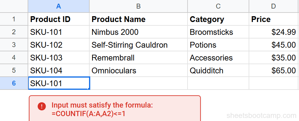
Using A:A (the full column) instead of a fixed range like A2:A12 means the rule still works when you add rows. The tradeoff is slightly slower evaluation on very large sheets. For most spreadsheets, the difference is unnoticeable.
Enforce a Text Pattern with REGEXMATCH
REGEXMATCH returns TRUE when a text string matches a regular expression pattern. Pair it with data validation to enforce specific formats.
Product Code Format (ABC-123)
=REGEXMATCH(A2, "^[A-Z]{3}-[0-9]{3}$")This requires exactly three uppercase letters, a hyphen, and three digits. Entries like SKU-101 pass. Entries like sku101, SK-1, or SKUU-1001 are rejected.
Email Address Format
=REGEXMATCH(B2, "^[a-zA-Z0-9._%+-]+@[a-zA-Z0-9.-]+\.[a-zA-Z]{2,}$")This validates basic email format: characters before the @, a domain, and a top-level domain of at least 2 characters. It catches typos like missing the @ symbol or forgetting the domain extension.
REGEXMATCH validates format, not existence. An email like fake@notreal.xyz passes the pattern check even though the address doesn’t exist. For true email verification, you need an external service.
Validate Based on Another Column
Custom formulas can reference any cell on the sheet, not just the cell being validated. This lets you create rules where one column’s valid input depends on another column’s value.
End Date Must Be After Start Date
If column B has start dates and column C has end dates, validate column C with:
=C2>B2This ensures the end date is always later than the start date in the same row. The row reference shifts automatically, so row 3 checks C3>B3, row 4 checks C4>B4, and so on.
Price Must Be Positive When Status Is Active
=OR(D2<>"Active", AND(D2="Active", C2>0))This allows any price when the status isn’t “Active”, but requires a positive price when it is. The OR function returns TRUE if either condition is met: the status isn’t Active, or the status is Active and the price is above zero.
Combine Multiple Conditions with AND/OR
The AND and OR functions let you stack multiple checks into a single validation formula.
AND: All Conditions Must Be True
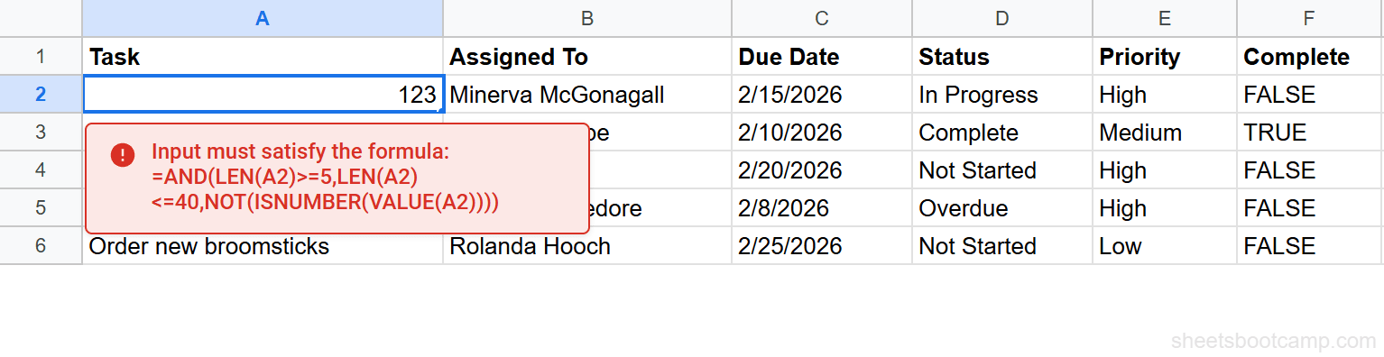
=AND(LEN(A2)>=5, LEN(A2)<=40, NOT(ISNUMBER(VALUE(A2))))This requires task names that are between 5 and 40 characters and are not purely numeric. All three conditions must pass for the entry to be accepted.
OR: At Least One Condition Must Be True
=OR(A2="N/A", ISNUMBER(A2))This allows either the text “N/A” or a number. Useful for optional numeric fields where users can type “N/A” to indicate the field doesn’t apply.
Common Mistakes
Formula Returns a Value Instead of TRUE/FALSE
A formula like =LEN(A2) returns a number, not TRUE or FALSE. Google Sheets treats any non-zero number as TRUE, so =LEN(A2) would allow all non-empty entries. Always include a comparison operator: =LEN(A2)<=40, =A2>0, =COUNTIF(A:A,A2)=1.
Wrong Cell Reference
If your apply-to range is A2:A12 and your formula references A1, every check is off by one row. The formula always references the first cell in the apply-to range.
Fix: Match the formula’s cell reference to the first cell in the range.
Missing Dollar Sign on Cross-Column References
When validating column C based on column B, write =C2>$B2 only if you’re applying validation across multiple columns. For single-column validation, dollar signs aren’t needed. The common error is adding dollar signs where they’re not needed, or leaving them out where they are.
Formula Doesn’t Account for Blank Cells
A formula like =REGEXMATCH(A2, "^[A-Z]{3}") returns an error on blank cells because REGEXMATCH can’t evaluate an empty string. Wrap it:
=OR(A2="", REGEXMATCH(A2, "^[A-Z]{3}-[0-9]{3}$"))This allows blank cells (the user hasn’t entered anything yet) while still enforcing the pattern for actual entries.
Tips
-
Test the formula in a regular cell first. Enter
=LEN(A2)<=40in an empty cell. If it returns TRUE for valid entries and FALSE for invalid ones, it will work in data validation. -
Use custom formulas alongside dropdowns. A dropdown restricts to a list, but custom formulas handle rules that lists can’t express. You can have both on different columns in the same sheet.
-
Combine with conditional formatting for visual feedback. Data validation blocks or warns on entry. Conditional formatting highlights cells that already contain invalid data (from before the rule was added, or from pasted data that bypasses validation).
-
Keep formulas simple. Complex formulas with multiple nested functions are harder to debug and slower to evaluate. If a rule needs five conditions, consider whether some of them belong in separate validation rules or in the sheet design itself.
-
Document your rules. Unlike dropdowns, custom formulas aren’t visible to users until they trigger a rejection. Add a note to the header cell or a helper text row explaining the input requirements.
Related Google Sheets Tutorials
- Data Validation in Google Sheets - Full guide to all validation rule types including dropdown, checkbox, and number criteria
- Create a Drop-Down List - Restrict input to a fixed set of values with dropdown menus
- Date Validation in Google Sheets - Restrict date entry with built-in and custom date rules
- Custom Formula Conditional Formatting - Use the same formula logic to highlight cells instead of blocking input
- IF with AND/OR - How AND, OR, and NOT work in formulas for multi-condition logic
Frequently Asked Questions
How do I use a custom formula in data validation in Google Sheets?
Select the cells, go to Data > Data validation, choose Custom formula is from the criteria dropdown, and enter a formula that returns TRUE or FALSE. TRUE allows the input, FALSE rejects it. The formula references the first cell in the apply-to range and shifts automatically for each row.
What formulas work with data validation in Google Sheets?
Any formula that returns TRUE or FALSE works. Common examples include comparison operators (=A2>0), text functions (=LEN(A2)<=50), date functions (=C2>=TODAY()), and logical functions like AND, OR, and NOT. You can combine multiple conditions in a single formula.
Why is my custom formula data validation not working?
The most common causes are: the formula doesn’t return TRUE or FALSE, the cell reference doesn’t match the first cell in the apply-to range, or the column reference isn’t locked when it should be. Test your formula in a regular cell first. If it returns TRUE for valid input and FALSE for invalid input, it will work in the validation rule.
Can I use REGEXMATCH in data validation?
Yes. REGEXMATCH returns TRUE or FALSE, making it ideal for pattern validation. For example, =REGEXMATCH(A2, "^[A-Z]{3}-[0-9]{3}$") ensures entries follow a specific format like ABC-123. This is useful for product codes, invoice numbers, and ID formats.
How do I prevent duplicate entries with data validation?
Use the formula =COUNTIF(A:A, A2)<=1 as your custom formula. COUNTIF counts how many times the value appears in the column. If the count exceeds 1, the entry is a duplicate and gets rejected. Apply the rule to the full input range.