Add or Subtract Days, Months, Years in Google Sheets
Learn how to add days to a date in Google Sheets and subtract days, months, or years. Includes EDATE for months, DATE for years, and deadline patterns.
Sheets Bootcamp
March 21, 2026
To add days to a date in Google Sheets, you add a number directly to the date cell. Date functions in Google Sheets treat dates as numbers, so =A2+90 moves a date forward by 90 days, and =A2-14 moves it back by 14. Adding months and years requires different functions, but the core concept is the same.
This guide covers adding and subtracting days, months, and years with step-by-step examples using an employee database. You’ll learn when to use arithmetic, when to use EDATE, and why adding 30 days is not the same as adding one month.
In This Guide
- Add Days to a Date
- Subtract Days from a Date
- Calculate 90-Day Review Dates: Step-by-Step
- Add Months with EDATE
- Add Years with DATE
- Why +30 Is Not the Same as +1 Month
- Practical Examples
- Common Errors and How to Fix Them
- Tips and Best Practices
- Related Google Sheets Tutorials
- Frequently Asked Questions
Add Days to a Date
Google Sheets stores dates as serial numbers. Adding a number to a date moves it forward by that many calendar days.
=D2+90Using Harry Potter’s hire date (8/1/2018) in cell D2, this returns 10/30/2018 — exactly 90 days later.
The number you add represents calendar days, including weekends and holidays. To add 7 days (one week), use =D2+7. To add 60 days, use =D2+60. There is no function needed. Dates are numbers, so arithmetic works directly.
You can also add a value from another cell. If cell F2 contains the number 90:
=D2+F2This keeps the day count flexible. Change the value in F2 and every formula that references it updates automatically.
Subtract Days from a Date
Subtracting days works the same way. Use the minus sign instead of plus.
=D2-14For Harry Potter’s hire date (8/1/2018), this returns 7/18/2018 — 14 days before the hire date. A common use: calculate a reminder date that falls 2 weeks before a deadline.
If you need to find how many days are between two dates, subtract one from the other:
=D2-D3Harry Potter’s hire date (8/1/2018) minus Hermione Granger’s hire date (9/1/2017) returns 334 — the number of days between the two dates. For more ways to measure date differences, see DATEDIF in Google Sheets.
Calculate 90-Day Review Dates: Step-by-Step
We’ll calculate 90-day review dates for every employee in the database using date arithmetic.
Set up your data
You need a table with a date column. The employee database has Hire Date in column D with 8 employees. The dates range from 9/1/2017 (Hermione Granger) to 3/22/2021 (Luna Lovegood).
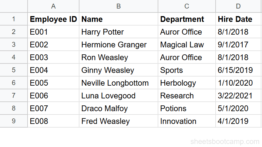
Add 90 days to calculate a review date
Select cell H2 (or any empty cell) and enter:
=D2+90For Harry Potter’s hire date of 8/1/2018, this returns 10/30/2018. The formula adds 90 calendar days to the date in D2.
If the result displays as a number like 43403 instead of a date, the cell is not formatted as a date. Select the cell, go to Format > Number > Date. For more formatting options, see how to format dates in Google Sheets.
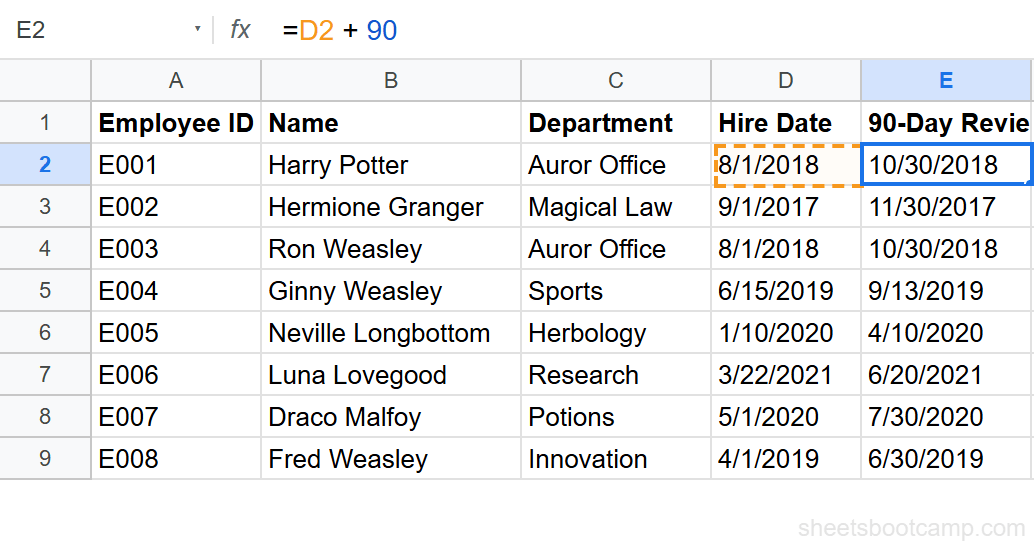
Add 6 months using EDATE
For a 6-month probation review, use EDATE instead of adding 180 days. In cell I2, enter:
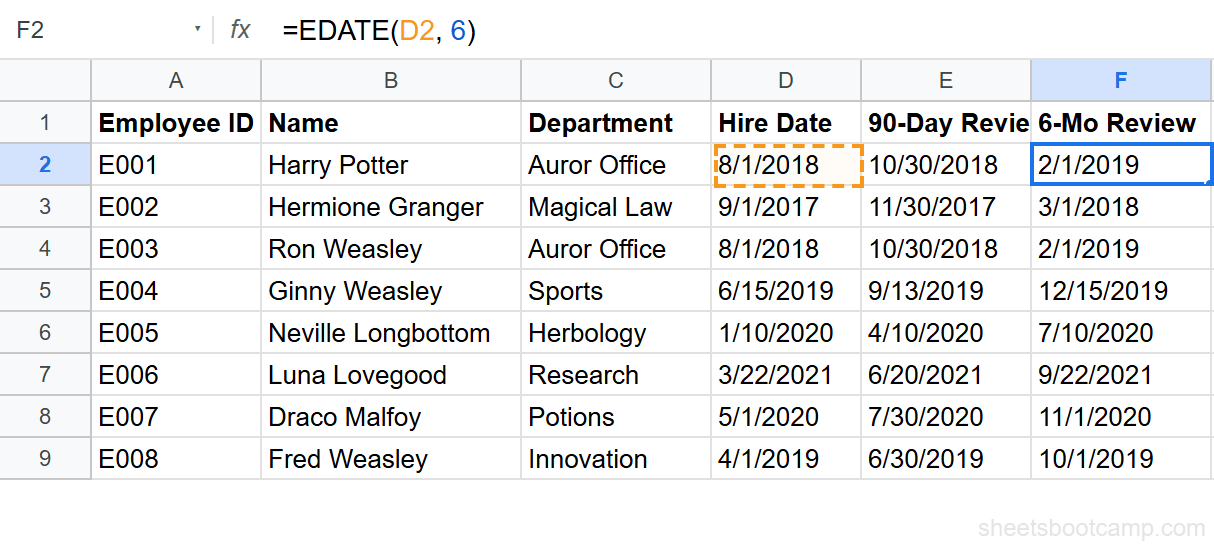
=EDATE(D2, 6)For Harry Potter’s hire date of 8/1/2018, this returns 2/1/2019. EDATE moves the date forward by exactly 6 months, keeping the same day of the month.
Copy the formulas down
Copy both formulas down through row 9. Each row calculates review dates based on its own hire date.
Spot-check the results:
- Hermione Granger — Hired 9/1/2017 — 90-day review: 11/30/2017, 6-month review: 3/1/2018
- Ginny Weasley — Hired 6/15/2019 — 90-day review: 9/13/2019, 6-month review: 12/15/2019
- Luna Lovegood — Hired 3/22/2021 — 90-day review: 6/20/2021, 6-month review: 9/22/2021
Add Months with EDATE
EDATE is the correct way to add or subtract months from a date. It handles varying month lengths automatically.
=EDATE(start_date, months)| Parameter | Description | Required |
|---|---|---|
| start_date | The date to start from | Yes |
| months | Number of months to add (positive) or subtract (negative) | Yes |
To add 6 months to Harry Potter’s hire date:
=EDATE(D2, 6)This returns 2/1/2019. To subtract 3 months from the same date:
=EDATE(D2, -3)This returns 5/1/2018 — three months before 8/1/2018.
EDATE preserves the day of the month when possible. If the target month has fewer days than the original day, EDATE returns the last day of that month. For example, =EDATE("1/31/2026", 1) returns 2/28/2026, not March 3.
Do not add 30 to a date when you mean “one month.” Adding 30 days to January 31 gives March 2, not February 28. EDATE handles month-length differences correctly.
Add Years with DATE
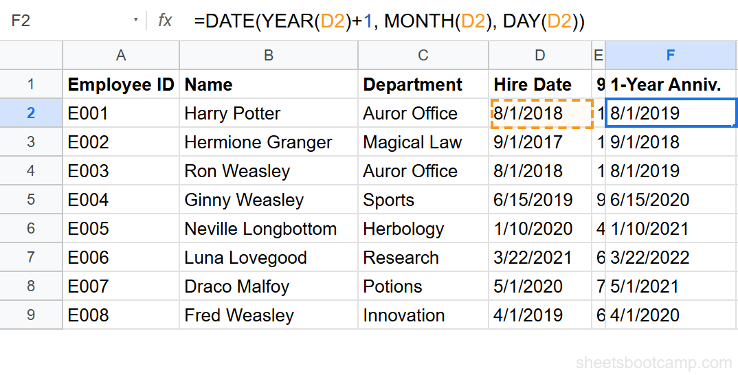
There is no EYEAR function in Google Sheets. To add years, use the DATE function with YEAR, MONTH, and DAY to reconstruct the date with a modified year.
=DATE(YEAR(D2)+1, MONTH(D2), DAY(D2))For Harry Potter’s hire date (8/1/2018), this returns 8/1/2019. The formula extracts the year (2018), adds 1, and rebuilds the date with the same month and day.
To add 5 years, change +1 to +5. To subtract 2 years, use -2:
=DATE(YEAR(D2)-2, MONTH(D2), DAY(D2))This returns 8/1/2016 — two years before Harry’s hire date.
To add both years and months at the same time, combine DATE and EDATE:
=EDATE(DATE(YEAR(D2)+1, MONTH(D2), DAY(D2)), 6)This adds 1 year and 6 months to the hire date, returning 2/1/2020.
DATE handles leap year edge cases. Adding 1 year to February 29, 2024 (a leap year) returns March 1, 2025, because February 29, 2025 does not exist. DATE overflows the day into the next month when the target date is invalid.
Why +30 Is Not the Same as +1 Month
This is the most common mistake with date arithmetic in Google Sheets. Adding 30 days and adding 1 month produce different results.
Consider January 31, 2026:
=DATE(2026,1,31)+30returns 3/2/2026 (30 calendar days later)=EDATE("1/31/2026", 1)returns 2/28/2026 (one month later, last day of February)
The difference is 2 days. For February dates, the gap gets wider in the other direction. Adding 30 days to February 1 gives March 3, but one month from February 1 is March 1.
When to use +30: You need exactly 30 calendar days. Examples: 30-day return policies, 30-day payment terms.
When to use EDATE: You need “one month from now” regardless of how many days that month has. Examples: monthly billing cycles, monthly review dates, subscription renewals.
For most business date calculations, EDATE is the right choice.
Practical Examples
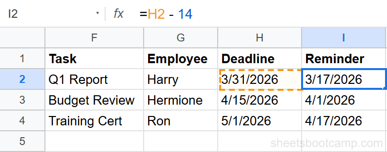
Deadline Reminder: 2 Weeks Before a Due Date
You have project deadlines in column E and need a reminder date 14 days before each one.
=E2-14If the deadline is 11/15/2026, this returns 11/1/2026. Pair this with conditional formatting to highlight rows where TODAY() has passed the reminder date but not the deadline.
Annual Anniversary Date
Calculate each employee’s next work anniversary:
=DATE(YEAR(TODAY()), MONTH(D2), DAY(D2))This builds a date using the current year and the month/day from the hire date. For Harry Potter (hired 8/1/2018), it returns 8/1/2026 if today is in 2026.
If the anniversary has already passed this year, add 1 to the year:
=IF(DATE(YEAR(TODAY()), MONTH(D2), DAY(D2))<TODAY(), DATE(YEAR(TODAY())+1, MONTH(D2), DAY(D2)), DATE(YEAR(TODAY()), MONTH(D2), DAY(D2)))This uses IF to check whether the anniversary date is in the past. If it is, the formula returns next year’s anniversary instead.
Days Until Next Anniversary
Combine the anniversary formula with TODAY() to count down:
=DATE(YEAR(TODAY()), MONTH(D2), DAY(D2))-TODAY()For Harry Potter with a hire anniversary of 8/1, this returns the number of days between today and 8/1/2026. If the result is negative, the anniversary already passed this year.
Common Errors and How to Fix Them
Result Shows a Number Instead of a Date
You enter =D2+90 and get 43403 instead of 10/30/2018. The formula is correct — the cell format is not set to display dates.
Fix: Select the cell, go to Format > Number > Date. The number converts to a readable date.
#VALUE! Error
A #VALUE! error means one of the cells contains text that looks like a date but is not a real date. This happens with imported data from CSV files or external sources.
Fix: Test with =ISNUMBER(D2). If it returns FALSE, the cell contains text. Convert it with =DATEVALUE(D2), then use the converted date in your formula.
Negative Date Result
Subtracting a later date from an earlier date returns a negative number. If =D2-D3 returns -334, the date in D3 is after the date in D2.
Fix: Swap the order: =D3-D2. Or use ABS to get the absolute value: =ABS(D2-D3).
Tips and Best Practices
-
Use EDATE for months, not +30. Month lengths vary from 28 to 31 days. EDATE accounts for this. Adding 30 is only correct when you need exactly 30 calendar days.
-
Use cell references for the number of days. Instead of
=D2+90, put 90 in a separate cell and reference it:=D2+F2. When the review period changes from 90 to 120 days, you update one cell instead of every formula. -
Lock ranges when copying formulas down. If your day count is in cell F1, use
=D2+$F$1so the reference to F1 stays fixed when you copy the formula to other rows. -
Pair date arithmetic with TODAY() for live countdowns.
=E2-TODAY()gives you the number of days until a deadline. Combine this with conditional formatting to highlight cells that drop below a threshold. -
Format result cells as dates before entering formulas. Select the output column, go to Format > Number > Date, then enter your formula. This prevents the serial-number display issue.
Related Google Sheets Tutorials
- Date Functions: The Complete Guide — All date functions in Google Sheets with syntax, examples, and error fixes
- TODAY and NOW Functions — Auto-updating dates for countdowns, age calculations, and timestamps
- DATEDIF Function Guide — Calculate differences between two dates in years, months, or days
- How to Format Dates — Custom date formats, locale settings, and display options
- Conditional Formatting Guide — Highlight upcoming deadlines and overdue dates with color rules
Frequently Asked Questions
How do I add 30 days to a date in Google Sheets?
Select an empty cell and enter =A2+30 where A2 contains your date. Google Sheets stores dates as numbers, so adding 30 moves the date forward by 30 calendar days. For Harry Potter’s hire date of 8/1/2018, =D2+30 returns 8/31/2018.
How do I add months to a date in Google Sheets?
Use the EDATE function. =EDATE(A2, 3) adds 3 months to the date in A2. EDATE handles varying month lengths correctly, so adding 1 month to January 31 returns February 28, not March 2. Use a negative number to subtract months: =EDATE(A2, -6).
How do I subtract dates in Google Sheets?
Subtract one date from another with =B2-A2. This returns the number of days between the two dates. To subtract a specific number of days from a date, use =A2-14 to go back 14 days. For months, use =EDATE(A2, -3) to go back 3 months.
Why is adding 30 days not the same as adding 1 month?
Months have different lengths. Adding 30 days to January 31 gives you March 2, not February 28. Adding 30 days to March 1 gives you March 31, but one month from March 1 is April 1. Use EDATE to add months correctly, and use +30 only when you need exactly 30 calendar days.
How do I add years to a date in Google Sheets?
Use the DATE function with YEAR, MONTH, and DAY: =DATE(YEAR(A2)+1, MONTH(A2), DAY(A2)). This adds exactly 1 year. Change the +1 to any number to add more years. For Harry Potter’s hire date of 8/1/2018, this returns 8/1/2019.