DATEDIF in Google Sheets: Calculate Days Between Dates
Learn how to use DATEDIF in Google Sheets to calculate days between dates, age from birthdate, and tenure. Covers all six units with step-by-step examples.
Sheets Bootcamp
March 19, 2026
DATEDIF in Google Sheets calculates the difference between two dates in years, months, or days. It is the go-to function for calculating age from a birthdate, employee tenure, or the exact span between any two dates.
DATEDIF does not appear in the autocomplete suggestions when you type in a cell. It is an undocumented function inherited from Lotus 1-2-3, but it works reliably in Google Sheets. This guide covers all six DATEDIF units, walks through calculating tenure and age step by step, and shows how to handle the common errors.
In This Guide
- DATEDIF Syntax and Parameters
- How to Calculate Tenure with DATEDIF: Step-by-Step
- DATEDIF Examples
- Common Errors and How to Fix Them
- DATEDIF vs Subtraction: When to Use Which
- Tips and Best Practices
- Related Google Sheets Tutorials
- Frequently Asked Questions
DATEDIF Syntax and Parameters
=DATEDIF(start_date, end_date, unit)| Parameter | Description | Required |
|---|---|---|
| start_date | The earlier date. Must come before end_date or you get a #NUM! error. | Yes |
| end_date | The later date. Often TODAY() for calculations relative to the current date. | Yes |
| unit | A text string specifying the output unit. See the table below. | Yes |
The Six DATEDIF Units
| Unit | Returns | Example (8/1/2018 to 2/18/2026) |
|---|---|---|
"Y" | Complete years | 7 |
"M" | Complete months (total) | 90 |
"D" | Total days | 2759 |
"YM" | Months remaining after complete years | 6 |
"MD" | Days remaining after complete months | 17 |
"YD" | Days remaining after complete years | 202 |
The first three units (Y, M, D) give you the full span in a single scale. The last three (YM, MD, YD) give you the leftover portion after subtracting the larger unit. Together, they let you build a display like “7 years, 6 months, 17 days.”
The start_date must be earlier than or equal to the end_date. If the start date comes after the end date, DATEDIF returns a #NUM! error. There is no optional argument to reverse this behavior.
How to Calculate Tenure with DATEDIF: Step-by-Step
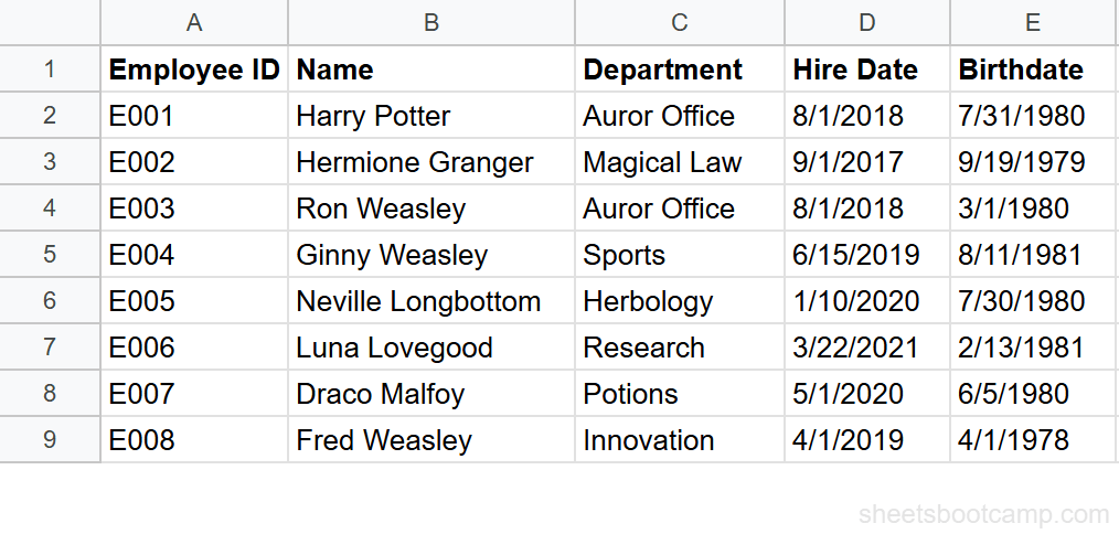
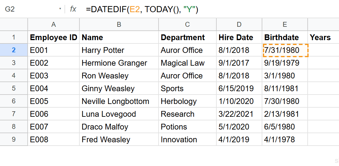
We’ll use the employee database to calculate how long each person has worked at the company. The data has 8 employees with Name in column B, Hire Date in column D, and Birthdate in column E.
Calculate tenure in complete years
Select an empty cell and enter:
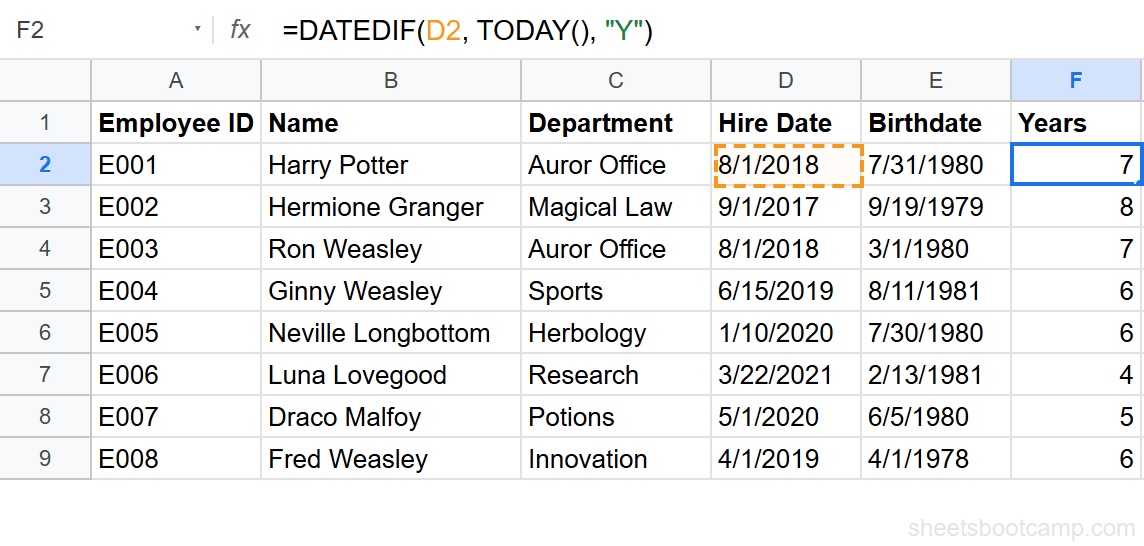
=DATEDIF(D2, TODAY(), "Y")D2 contains Harry Potter’s hire date (8/1/2018). The "Y" unit returns the number of complete years between that date and today. As of February 2026, this returns 7.
See all three primary units
Enter two more DATEDIF formulas using the same start and end dates but with different units:
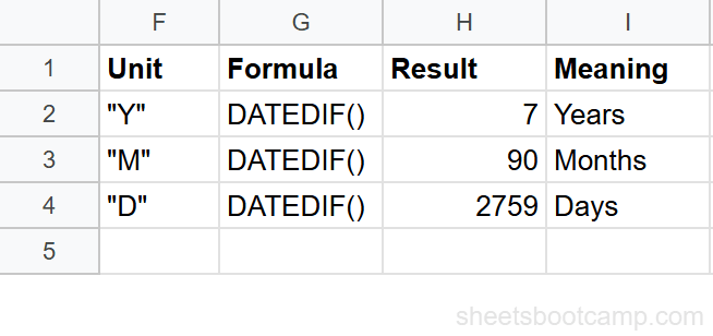
=DATEDIF(D2, TODAY(), "M")=DATEDIF(D2, TODAY(), "D")The "M" unit returns 90 total months. The "D" unit returns 2759 total days. Each unit gives you the same date span measured on a different scale.
Use "D" when you need an exact day count for project timelines or billing cycles. Use "Y" or "M" when the result needs to be human-readable for reports and dashboards.
Combine units for years, months, and days
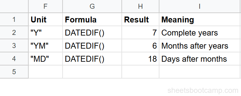
The "YM" unit returns the remaining months after complete years. The "MD" unit returns the remaining days after complete months. Combine them with the ampersand operator (&) to build a text string:
=DATEDIF(D2, TODAY(), "Y") & " years, " & DATEDIF(D2, TODAY(), "YM") & " months, " & DATEDIF(D2, TODAY(), "MD") & " days"This returns a string like “7 years, 6 months, 17 days” (the exact values depend on today’s date). Three separate DATEDIF calls feed into a single readable output.
For more on building text strings with the ampersand operator, see text functions in Google Sheets.
Calculate age from birthdate
The same DATEDIF pattern works for age. Enter:
=DATEDIF(E2, TODAY(), "Y")E2 contains Harry Potter’s birthdate (7/31/1980). This returns 45 as of February 2026. Copy the formula down through all 8 employees.
Spot-check a few rows:
- Hermione Granger (born 9/19/1979) — age 46
- Fred Weasley (born 4/1/1978) — age 47
- Luna Lovegood (born 2/13/1981) — age 45
Copy formulas down for all employees
Select the tenure formula cell and drag the fill handle down through row 9 to calculate tenure for all 8 employees. Do the same for the age formula. Each row references its own Hire Date and Birthdate, so the results update per employee. Hermione Granger shows the longest tenure at 8 years (hired 9/1/2017).
DATEDIF Examples
Example 1: Days Until a Deadline
You have a project deadline in cell B2 and want to know how many days remain. Use TODAY() as the start date and the deadline as the end date:
=DATEDIF(TODAY(), B2, "D")If B2 contains 6/30/2026, this returns the total number of calendar days from today until June 30. Once the deadline passes, the formula returns a #NUM! error because TODAY() becomes the later date. Wrap it in IFERROR to handle that:
=IFERROR(DATEDIF(TODAY(), B2, "D"), "Past due")Example 2: Display “X Years, Y Months” for All Employees
For a report-ready tenure column, combine "Y" and "YM" into a formatted string:
=DATEDIF(D2, TODAY(), "Y") & " yr " & DATEDIF(D2, TODAY(), "YM") & " mo"Results for the employee database:
- Harry Potter (hired 8/1/2018): 7 yr 6 mo
- Hermione Granger (hired 9/1/2017): 8 yr 5 mo
- Neville Longbottom (hired 1/10/2020): 6 yr 1 mo
- Luna Lovegood (hired 3/22/2021): 4 yr 10 mo
The "Y" unit gives complete years. The "YM" unit gives the remaining months. Together they tell the full story without rounding.
Example 3: The YD Unit for Anniversary Tracking
The "YD" unit returns the number of days since the last anniversary of the start date. Use it to see how far into the current year of service an employee is:
=DATEDIF(D2, TODAY(), "YD")For Harry Potter (hired 8/1/2018), this returns the number of days since his last work anniversary on 8/1/2025. If today is February 18, 2026, the result is 202 days into his 8th year of service.
Common Errors and How to Fix Them
#NUM! Error
DATEDIF returns #NUM! when the start date is after the end date. This is the most common DATEDIF error.
=DATEDIF(TODAY(), D2, "Y")This breaks because TODAY() (2026) comes after Harry Potter’s hire date (2018). Swap the arguments:
=DATEDIF(D2, TODAY(), "Y")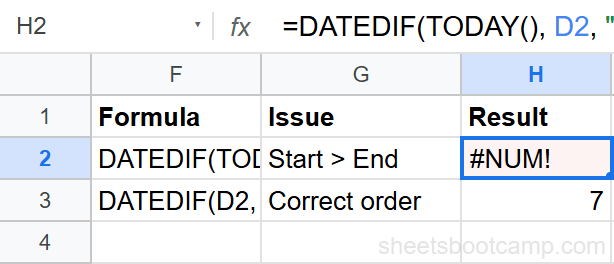
If your data might have dates in either order (e.g., comparing two dates where either could be earlier), use IFERROR to catch the error:
=IFERROR(DATEDIF(A2, B2, "D"), DATEDIF(B2, A2, "D"))This tries A2 as the start date first. If that produces a #NUM! error, it swaps and tries B2 as the start date instead.
#VALUE! Error
A #VALUE! error means one of the date arguments is not a valid date. The most common cause: the cell contains text that looks like a date but is not recognized by Google Sheets.
Test with =ISNUMBER(D2). If it returns FALSE, the cell is text. Fix it with =DATEVALUE(D2) to convert the text to a proper date, then use that converted value in your DATEDIF formula.
This happens frequently with dates imported from CSV files or pulled with IMPORTRANGE.
MD Unit Quirks
The "MD" unit (days remaining after complete months) can produce unexpected results near month boundaries. Google Sheets’ implementation occasionally returns negative numbers or miscounts when the start day is later in the month than the end day.
For example, DATEDIF from 1/31/2026 to 3/1/2026 with "MD" might return an unexpected value instead of the 1 day you would expect. If your results look wrong with "MD", cross-check with =DAY(end_date) - DAY(start_date) and adjust as needed.
The "MD" quirk is a known issue in both Google Sheets and Excel. For most use cases, "Y" and "YM" are reliable. Only "MD" has these edge cases. If you need exact remaining days and the "MD" result looks suspicious, verify it manually.
DATEDIF vs Subtraction: When to Use Which
Subtracting two dates in Google Sheets gives you the number of days between them:
=B2-A2This is faster to type than DATEDIF with the "D" unit, and it works in both directions (negative result if A2 is later). So when do you need DATEDIF?
Use subtraction when:
- You need total days and nothing else
- You want the result to work regardless of date order (negative values are acceptable)
- You are feeding the result into another calculation
Use DATEDIF when:
- You need years, months, or a combined display (Y, M, YM, MD)
- You are calculating age from a birthdate where complete years matter
- You want “7 years, 6 months” instead of “2759 days”
Subtraction is a shortcut for day counts. DATEDIF is the right tool when you need to express the date difference in human-readable units.
Tips and Best Practices
-
Always use TODAY() as the end date for age and tenure. Hardcoding a date means your formula goes stale tomorrow. TODAY() recalculates every time the sheet opens.
-
Type DATEDIF manually. It will not appear in autocomplete or the function list. Type
=DATEDIF(and the formula works despite the lack of suggestions. Google Sheets inherited this function from Lotus 1-2-3 and never added it to the official documentation. -
Combine Y and YM for the most useful display. Total months (
"M") or total days ("D") are useful for calculations, but reports look better with “7 years, 6 months.” Use the combined formula pattern from Step 3. -
Wrap DATEDIF in IFERROR when date order is uncertain. User-entered dates might be in the wrong order.
=IFERROR(DATEDIF(A2, B2, "D"), "Check dates")prevents #NUM! errors from breaking your sheet. -
Avoid the MD unit for precise calculations. The
"MD"unit has known quirks near month boundaries. If you need days remaining after months, cross-check with=DAY(end_date) - DAY(start_date)to confirm accuracy. See adding and subtracting dates for alternative approaches.
Related Google Sheets Tutorials
- Date Functions: The Complete Guide — Overview of all date functions including TODAY, EDATE, NETWORKDAYS, and DATEVALUE
- TODAY and NOW Functions — Auto-updating current date and time, plus patterns for combining with DATEDIF
- How to Add and Subtract Dates — EDATE, date math, and working with date intervals
- How to Format Dates — Custom date formats, locale settings, and display options
- IF Statements in Google Sheets — Build conditional logic and IFERROR wrappers for date formulas
Frequently Asked Questions
Why does DATEDIF not autocomplete in Google Sheets?
DATEDIF is an undocumented function inherited from Lotus 1-2-3. Google Sheets supports it but does not include it in the autocomplete suggestions or the function list. You need to type the full formula manually, and it works the same as any other function.
How do I calculate age from a birthdate in Google Sheets?
Use =DATEDIF(birthdate, TODAY(), "Y") where birthdate is the cell containing the date of birth. The "Y" unit returns the number of complete years, which is the person’s current age. The formula updates automatically each day because of TODAY().
What is the difference between DATEDIF units M and YM?
The "M" unit returns the total number of complete months between two dates. The "YM" unit returns only the remaining months after subtracting complete years. For a span of 2 years and 3 months, "M" returns 27 while "YM" returns 3.
Can DATEDIF calculate hours or minutes between dates?
No. DATEDIF works with whole dates only and its smallest unit is days ("D"). For hours or minutes, subtract the two date-time values and multiply by 24 for hours or 1440 for minutes. Make sure both cells contain date-time values, not dates alone.
How do I fix the #NUM! error in DATEDIF?
The #NUM! error means the start date is after the end date. DATEDIF requires the first argument to be the earlier date. Swap the arguments, or wrap the formula in IFERROR: =IFERROR(DATEDIF(A2, B2, "D"), "Check dates") to handle cases where the order is uncertain.