How to Format Dates in Google Sheets
Learn to format dates in Google Sheets with the Format menu, custom number formats, and the TEXT function. Includes all format codes and common fixes.
Sheets Bootcamp
March 20, 2026
When you format dates in Google Sheets, you control how dates appear without changing the underlying values. Google Sheets stores every date as a serial number internally, so the same date can display as “8/1/2018,” “August 1, 2018,” or “2018-08-01” depending on the format you apply. This guide covers three methods for changing date formats, a full reference of format codes, and fixes for common date display problems.
In This Guide
- Three Ways to Format Dates
- Method 1: Built-in Date Formats (Format Menu)
- Method 2: Custom Number Format
- Apply a Custom Date Format: Step-by-Step
- Method 3: TEXT Function
- Date Format Code Reference
- Common Date Format Patterns
- Common Problems and Fixes
- Tips and Best Practices
- Related Google Sheets Tutorials
- Frequently Asked Questions
Three Ways to Format Dates
Google Sheets gives you three methods to change how dates display:
- Format > Number menu — Pick a built-in date format. Fast, but limited to a few preset options.
- Custom number format — Write your own format pattern using codes like
YYYY-MM-DD. Full control over the display while keeping the date value intact. - TEXT function — Convert a date to a text string in any format. Useful inside formulas, but the result is text and no longer works in date calculations.
Methods 1 and 2 change the display format only. The cell still contains a date, and you can use it in DATEDIF, TODAY, or any other date function. Method 3 produces a text string, so choose it only when you need formatted text for labels, reports, or concatenation.
Method 1: Built-in Date Formats (Format Menu)
The fastest way to change date format in Google Sheets:
- Select the cells containing dates
- Go to Format > Number
- Choose one of the built-in options:
| Menu Option | Example Output |
|---|---|
| Date | 12/31/2018 |
| Time | 3:59:00 PM |
| Date time | 12/31/2018 3:59:00 PM |
| Duration | 24:01:00 |
The built-in Date format uses your spreadsheet’s locale setting. For U.S. locale, that is M/D/YYYY. For U.K. locale, it is DD/MM/YYYY.
The locale setting affects all default date formats in the spreadsheet. To change your locale, go to File > Settings > General > Locale. This affects the entire spreadsheet, not individual cells.
The built-in formats work for quick formatting but do not let you customize the pattern. For formats like “Aug 2018” or “2018-08-01,” use a custom number format.
Method 2: Custom Number Format
Custom number formats let you build any date display pattern using format codes. The date value stays intact — only the visual display changes.
To apply a custom date format:
- Select the cells containing dates
- Go to Format > Number > Custom number format
- Type a format pattern in the text field (e.g.,
MMMM D, YYYY) - Click Apply
The format codes control each component of the date:
DorDD— Day of the monthMorMM— Month numberMMMorMMMM— Month name (short or full)YYorYYYY— Year (two-digit or four-digit)DDDorDDDD— Day name (short or full)
You can combine these codes with any separator: slashes, hyphens, commas, spaces. Google Sheets reads the codes and displays the rest as literal characters.
Apply a Custom Date Format: Step-by-Step
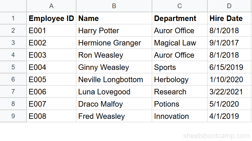
We’ll format the Hire Date column in the employee database from the default 8/1/2018 to the long date format August 1, 2018.
Sample Data
The employee database has Employee ID in column A, Name in column B, Department in column C, and Hire Date in column D, with 8 employees.
Select the date cells
Click cell D2 and drag down to D9 to select all 8 hire dates. You can also click the column D header if the entire column contains dates.
Open the Format menu
Go to Format > Number in the menu bar. At the bottom of the submenu, click Custom number format. A dialog box opens with a text field for your format pattern.
Enter the format pattern
Type MMMM D, YYYY in the text field. This tells Google Sheets to display the full month name, the day without a leading zero, a comma, and the four-digit year. Click Apply.
The dates change from 8/1/2018 to August 1, 2018. Harry Potter’s hire date now reads August 1, 2018 instead of 8/1/2018. Hermione Granger’s reads September 1, 2017.
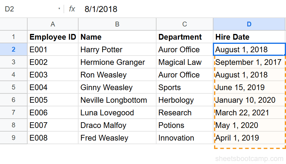
Verify the underlying value
Click any formatted cell and check the formula bar. It still shows the original date value (e.g., 8/1/2018), confirming the data is unchanged. The custom format affects the display only. You can still use these cells in date calculations like =DATEDIF(D2, TODAY(), "Y").
Custom number formats change the display, not the value. If you sort a column of formatted dates, Google Sheets sorts by the underlying date serial numbers, not the display text. This means sorting always works correctly regardless of the format.
Method 3: TEXT Function
The TEXT function converts a date value into a text string in any format you specify. Use this when you need formatted date text inside a formula, concatenation, or a label.
=TEXT(date_value, format_pattern)| Parameter | Description | Required |
|---|---|---|
| date_value | A cell reference or date value | Yes |
| format_pattern | A format string using date codes (in quotes) | Yes |
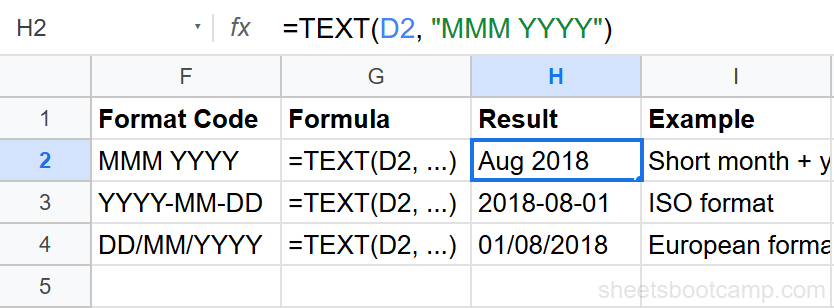
Using Harry Potter’s hire date in cell D2 (8/1/2018):
=TEXT(D2, "MMM YYYY")This returns Aug 2018 as a text string.
=TEXT(D2, "YYYY-MM-DD")This returns 2018-08-01 in ISO 8601 format.
=TEXT(D2, "DD/MM/YYYY")This returns 01/08/2018 in European day-first format.
TEXT returns a text string, not a date. You cannot use TEXT results in date arithmetic like =TEXT(D2, "YYYY-MM-DD") + 30. If you need to format a date for display but still use it in calculations, apply a custom number format instead.
The TEXT function is especially useful with concatenation. To build a sentence like “Hired: August 1, 2018,” use:
="Hired: " & TEXT(D2, "MMMM D, YYYY")This returns Hired: August 1, 2018. For more on combining text and values, see Google Sheets text functions.
Date Format Code Reference
Every code below works in both custom number formats and the TEXT function.
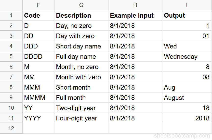
| Code | Description | Example (8/1/2018) |
|---|---|---|
D | Day of month, no leading zero | 1 |
DD | Day of month with leading zero | 01 |
DDD | Abbreviated day name | Wed |
DDDD | Full day name | Wednesday |
M | Month number, no leading zero | 8 |
MM | Month number with leading zero | 08 |
MMM | Abbreviated month name | Aug |
MMMM | Full month name | August |
YY | Two-digit year | 18 |
YYYY | Four-digit year | 2018 |
The letter case does not matter for custom number formats. yyyy-mm-dd, YYYY-MM-DD, and Yyyy-Mm-Dd all produce the same output. In the TEXT function, case also does not matter.
Common Date Format Patterns
Here are the most-used format patterns with their output, using Harry Potter’s hire date (8/1/2018):
| Pattern | Output | Use Case |
|---|---|---|
M/D/YYYY | 8/1/2018 | U.S. standard |
DD/MM/YYYY | 01/08/2018 | European standard |
YYYY-MM-DD | 2018-08-01 | ISO 8601, databases, sorting |
MMM D, YYYY | Aug 1, 2018 | Short labels |
MMMM D, YYYY | August 1, 2018 | Formal documents |
DDDD, MMMM D, YYYY | Wednesday, August 1, 2018 | Full display with day name |
MMM YYYY | Aug 2018 | Month-year only |
MM/YYYY | 08/2018 | Month-year with numbers |
DDD, MMM D | Wed, Aug 1 | Short calendar-style |
The YYYY-MM-DD format is the best choice for data that needs to sort correctly as text, since the year comes first.
Common Problems and Fixes
Date Displays as a Number (e.g., 43313)
Google Sheets stores dates as serial numbers counting from December 30, 1899. Day 1 is December 31, 1899. If a cell shows 43313 instead of a date, the cell is formatted as a plain number.
Fix: Select the cell, go to Format > Number > Date. The number 43313 becomes 8/1/2018.
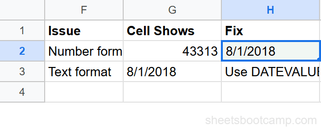
This happens when you paste data from external sources or when a formula returns a date serial number into a cell that is formatted as a number.
Text That Looks Like a Date But Is Not
Sometimes a cell shows 8/1/2018 but Google Sheets treats it as text instead of a date. You can tell because the text is left-aligned (dates are right-aligned by default) and date functions return errors.
Fix: Use the DATEVALUE function to convert the text to a real date:
=DATEVALUE(D2)This returns the date serial number. Format the result cell as a date. If you need to fix an entire column, use DATEVALUE in a helper column and paste the values back.
A quick way to check if a cell contains a real date: select it and look at the formula bar. If the formula bar shows a date format and the cell is right-aligned, it is a real date. If the cell is left-aligned, it is likely text. You can also try =ISNUMBER(D2) — real dates return TRUE, text returns FALSE.
Date Changes When Pasting Between Locales
If you copy a date from a spreadsheet set to U.S. locale (M/D/YYYY) and paste it into one set to U.K. locale (DD/MM/YYYY), the date can be misinterpreted. For example, 3/5/2024 becomes May 3rd instead of March 5th.
Fix: Use the YYYY-MM-DD format when sharing data between spreadsheets with different locale settings. This format is unambiguous because the year comes first.
Tips and Best Practices
-
Use custom number formats over TEXT when possible. Custom formats preserve the date value so you can still sort, filter, and calculate with the cell. TEXT converts the date to a string, which limits what you can do with it afterward.
-
Standardize on
YYYY-MM-DDfor data exports. The ISO format sorts correctly as text, avoids locale confusion, and is recognized by databases and APIs. Apply it as a custom number format before exporting. -
Check your spreadsheet locale before formatting. Go to File > Settings > General to see your locale. The default date format and month/day order depend on this setting. Changing the locale affects all default date displays in the spreadsheet.
-
Use conditional formatting to highlight date ranges. You can set up rules that color-code dates based on whether they are past, present, or future. Combine this with the custom date format for clear date-based dashboards.
-
Format the column before entering data. If you apply a custom date format to an empty column first, every date you enter appears in that format immediately. This saves time compared to formatting after the fact.
Related Google Sheets Tutorials
- Date Functions: The Complete Guide — Overview of all date functions including DATEDIF, EDATE, NETWORKDAYS, and more
- TODAY and NOW Functions — Get the current date or timestamp that updates automatically
- DATEDIF Function: Calculate Days Between Dates — Calculate years, months, or days between two dates
- Add or Subtract Days, Months, and Years — Date arithmetic with EDATE, direct addition, and more
- Text Functions: The Complete Guide — Use TEXT, CONCATENATE, and other text functions to build formatted strings
Frequently Asked Questions
How do I change the date format in Google Sheets?
Select the cells containing dates, go to Format > Number, and pick a built-in date format. For a specific pattern like YYYY-MM-DD, choose Custom number format and enter the format codes yourself.
What is the difference between formatting a date and using the TEXT function?
Formatting changes how a date looks but keeps the underlying date value intact. The TEXT function converts the date to a text string in the specified format. Formatted dates still work in date calculations. TEXT results do not.
Why does my date show as a number like 43313?
Google Sheets stores dates as serial numbers counting from December 30, 1899. If a cell shows a number like 43313, the cell is formatted as a plain number instead of a date. Select the cell, go to Format > Number > Date, and the date appears.
What format codes does Google Sheets use for dates?
Google Sheets uses D for day, M for month, and Y for year. DD adds a leading zero, DDD shows the short day name (Mon), DDDD shows the full name (Monday). MM adds a leading zero, MMM shows the short month (Jan), MMMM shows the full name (January). YY gives a two-digit year and YYYY a four-digit year.
Can I format dates differently in different cells?
Yes. Each cell can have its own number format. Select the cells you want to change, apply a custom date format, and leave the rest of the column in a different format. You can also use the TEXT function to output different formats in separate columns.