TODAY and NOW Functions in Google Sheets
Learn how to use the TODAY function in Google Sheets to calculate age, tenure, and days until a deadline. Covers NOW for timestamps and time tracking.
Sheets Bootcamp
March 18, 2026
The TODAY function in Google Sheets returns the current date, and it updates every time your spreadsheet recalculates. Combined with date functions like DATEDIF, EDATE, and IF, TODAY turns static dates into live calculations for age, tenure, countdowns, and overdue checks. This guide covers how TODAY and NOW work, when to use each one, and how to build formulas that stay current without manual updates.
In This Guide
- TODAY vs NOW: When to Use Each
- Syntax
- How to Use TODAY and NOW: Step-by-Step
- Practical Examples
- Common Errors and How to Fix Them
- Tips and Best Practices
- Related Google Sheets Tutorials
- Frequently Asked Questions
TODAY vs NOW: When to Use Each
Both functions return the current moment, but they serve different purposes.
TODAY() returns the current date as a date value with no time component. Use it for:
- Calculating age or tenure in years
- Counting days until a deadline
- Checking if a date has passed
- Conditional formatting rules that compare cells to the current date
NOW() returns the current date and time as a datetime value. Use it for:
- Logging when an action happened
- Tracking elapsed hours or minutes
- Time-stamping entries in a shared sheet
The practical difference: =TODAY() returns 3/18/2026. =NOW() returns 3/18/2026 2:45:00 PM. If your formula only needs the date, use TODAY. If you need hours and minutes, use NOW.
Syntax
Both functions take zero arguments.
=TODAY()| Parameter | Description | Required |
|---|---|---|
| (none) | TODAY takes no arguments. The parentheses are required but stay empty. | N/A |
=NOW()| Parameter | Description | Required |
|---|---|---|
| (none) | NOW takes no arguments. The parentheses are required but stay empty. | N/A |
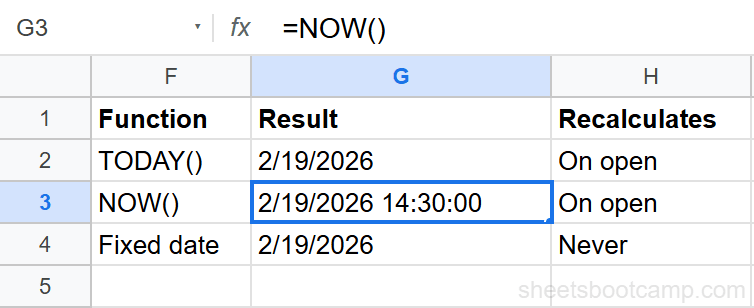
TODAY and NOW are volatile functions. They recalculate every time any cell changes, every time you open the spreadsheet, and at regular intervals while the sheet is open. You cannot freeze the value inside the formula. To lock a date, paste the cell as value only (Ctrl+Shift+V).
How to Use TODAY and NOW: Step-by-Step
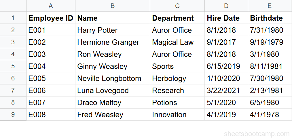
We’ll use an employee database with 8 employees. The table has Name in column A, Employee ID in column B, Department in column C, Hire Date in column D, and Birthdate in column E.
Sample Data
The employee database includes Harry Potter (hired 8/1/2018), Hermione Granger (hired 9/1/2017), Ron Weasley (hired 8/1/2018), and 5 more employees across departments like Auror Office, Magical Law, and Herbology.
Review your employee data
Open the spreadsheet with employee records. Column D contains Hire Dates ranging from 9/1/2017 (Hermione Granger) to 3/22/2021 (Luna Lovegood). Column E contains Birthdates. You’ll use these dates with TODAY to calculate live tenure and age values.
Enter the TODAY function
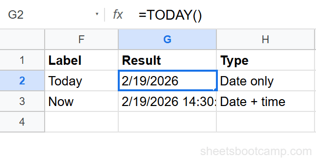
Select cell G2 and enter:
=TODAY()The cell displays the current date (for example, 3/18/2026). This value changes each day without any manual input. Every other formula that references G2 will use today’s date.
Calculate tenure with DATEDIF and TODAY
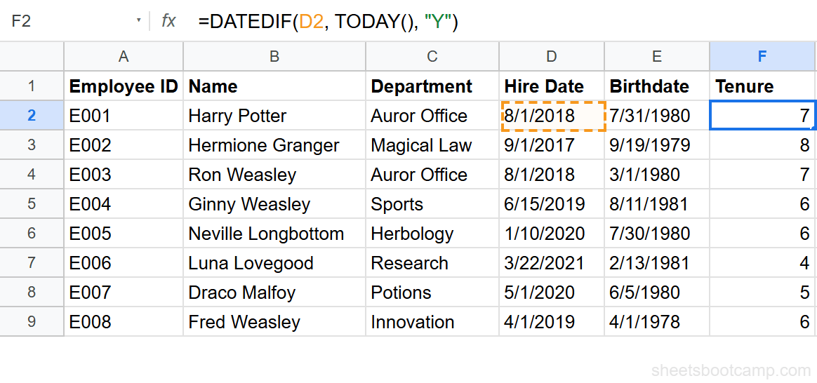
Select cell H2 and enter:
=DATEDIF(D2, TODAY(), "Y")This returns 7 for Harry Potter, meaning 7 full years have passed since his hire date of 8/1/2018. DATEDIF calculates the difference between two dates, and TODAY supplies the end date so the result stays current. Copy the formula down to H9 to calculate tenure for all 8 employees.
Change the third argument in DATEDIF to "M" for months or "D" for days. =DATEDIF(D2, TODAY(), "M") returns the total months of tenure instead of years.
Add a NOW timestamp
Select cell I2 and enter:
=NOW()The cell displays the current date and time, such as 3/18/2026 2:45:00 PM. If you only see a date, select the cell and go to Format > Number > Date time to reveal the time portion.
Build a conditional tenure check
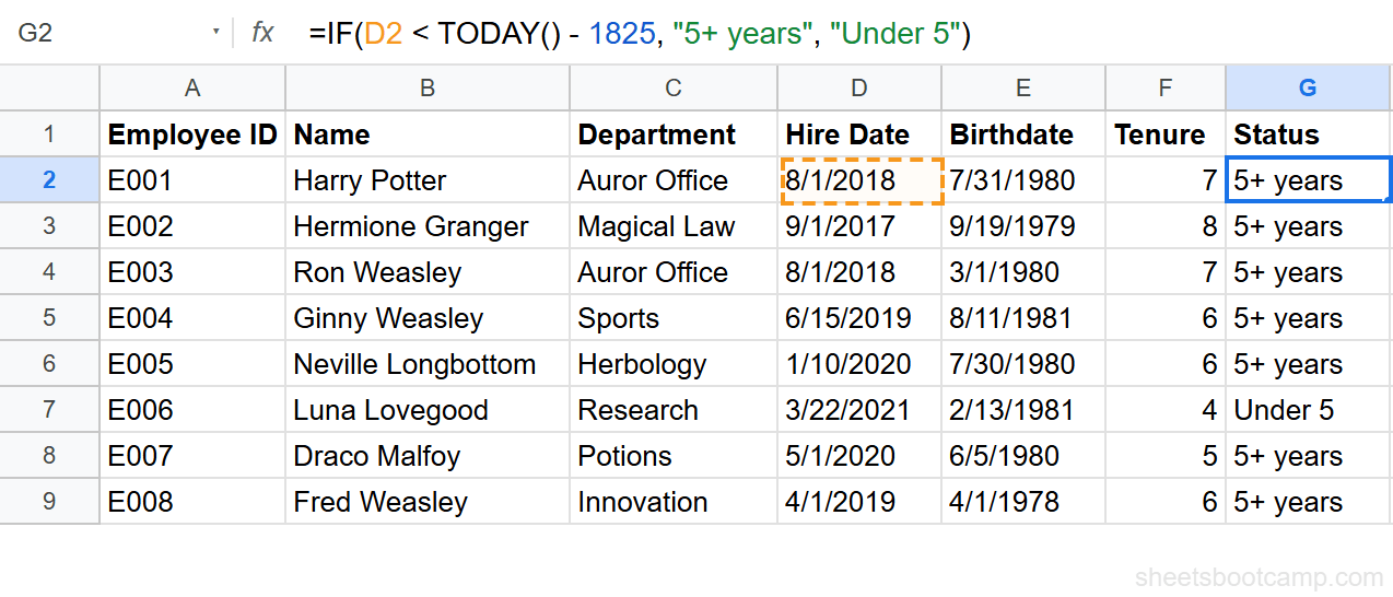
Select cell J2 and enter:
=IF(D2 < TODAY() - 1825, "Over 5 Years", "Under 5 Years")This checks whether the hire date is more than 1,825 days ago (approximately 5 years). Harry Potter’s hire date of 8/1/2018 is well over 5 years ago, so the formula returns Over 5 Years. Copy down to J9. Hermione Granger, Ron Weasley, Ginny Weasley, Neville Longbottom, Draco Malfoy, and Fred Weasley all return “Over 5 Years.” Only Luna Lovegood (hired 3/22/2021) returns “Under 5 Years” since her hire date falls within the 1,825-day window.
This pattern works well with IF formulas for any date-based threshold check: overdue invoices, expiring contracts, or upcoming renewals.
Practical Examples
Calculate Age from Birthdate
Use DATEDIF with TODAY to calculate each employee’s age in years:
=DATEDIF(E2, TODAY(), "Y")For Harry Potter (born 7/31/1980), this returns 45. For Fred Weasley (born 4/1/1978), it returns 47. The result updates on each employee’s birthday.
Days Until a Target Date
Count the days remaining until a specific date. If cell K1 contains a project deadline of 6/30/2026:
=K1 - TODAY()On 3/18/2026, this returns 104 — the number of days between today and the deadline. If the deadline has passed, the result is negative. Format the cell as a number (not a date) to see the day count.
Overdue Flag with Conditional Formatting
You can use TODAY inside a conditional formatting custom formula. To highlight any hire date older than 7 years:
- Select the Hire Date column (D2:D9)
- Go to Format > Conditional formatting
- Set the format rule to Custom formula is
- Enter
=D2 < TODAY() - 2555
Cells with hire dates more than 2,555 days ago (approximately 7 years) turn the color you selected. The rule recalculates daily because TODAY updates automatically.
Common Errors and How to Fix Them
Date Displays as a Number
You enter =TODAY() and the cell shows 46094 instead of a date. Google Sheets stores dates as serial numbers (days since 12/30/1899). The cell is formatted as a number.
Fix: Select the cell, go to Format > Number > Date, and the serial number displays as a readable date.
Math Produces a Date Instead of a Number
You enter =TODAY() - D2 expecting a number of days, but the cell shows a date like 1/14/1933.
Fix: The result cell is formatted as a date. Select it, go to Format > Number > Number, and you see the day count (for example, 2,786 days).
Date math in Google Sheets always produces a number. Whether that number displays as a date or an integer depends on the cell format. If your result looks wrong, check the format first.
NOW Shows Only a Date
You enter =NOW() but the cell shows 3/18/2026 with no time. The time data is there, but the cell format hides it.
Fix: Select the cell and choose Format > Number > Date time. The full datetime appears.
Tips and Best Practices
-
Use TODAY for date-only calculations. TODAY returns midnight (no time component), which prevents rounding errors when subtracting dates. NOW includes the time, which can produce fractional day differences.
-
Paste as value to freeze a date. Select the cell with
=TODAY(), press Ctrl+C, then Ctrl+Shift+V to paste the value. This replaces the formula with a static date that will not change. -
Combine TODAY with date arithmetic. Add or subtract days directly:
=TODAY() + 30returns the date 30 days from now.=TODAY() - 90returns the date 90 days ago. No extra functions needed. -
Use number formatting to control display. A single TODAY formula can display as “March 18, 2026” or “03/18/26” or “2026-03-18” depending on the cell format. The underlying value is the same.
-
Avoid NOW in date-only formulas. If you use NOW where TODAY would work, the time portion creates fractional differences.
=NOW() - D2might return 2786.63 instead of a clean integer. Stick to TODAY unless you need the time.
Related Google Sheets Tutorials
- Google Sheets Date Functions: The Complete Guide — Full reference covering TODAY, NOW, DATEDIF, EDATE, NETWORKDAYS, and more
- DATEDIF Function in Google Sheets — Calculate the difference between two dates in days, months, or years
- How to Format Dates in Google Sheets — Control how dates display using built-in and custom formats
- Add or Subtract Days, Months, Years — Date arithmetic formulas for shifting dates forward or backward
- IF Function in Google Sheets — Build conditional logic for date-based checks and labels
Frequently Asked Questions
What is the difference between TODAY and NOW in Google Sheets?
TODAY returns the current date without a time component. NOW returns both the current date and the current time. Use TODAY for date calculations like age or tenure. Use NOW when you need a timestamp that includes hours and minutes.
Does the TODAY function update automatically?
Yes. TODAY recalculates every time Google Sheets recalculates, which happens when you edit any cell, open the spreadsheet, or trigger a refresh. You cannot prevent it from updating. If you need a fixed date, paste the value using Ctrl+Shift+V.
Can I use TODAY in an IF formula?
Yes. You can combine TODAY with IF to run date-based checks. For example, =IF(C2 < TODAY() - 1825, "Over 5 Years", "Under 5 Years") compares a hire date to a date 5 years ago and returns a label.
How do I get the current date in Google Sheets without it changing?
Enter =TODAY() in a cell, then immediately copy the cell and paste as value only using Ctrl+Shift+V. This replaces the formula with a static date that will not update. You can also type the date manually.
Why does my NOW function only show a date without the time?
The cell is formatted as a date. Select the cell, go to Format > Number > Date time, and the time component becomes visible. NOW always returns both date and time, but the cell format controls what you see.