WEEKDAY Function in Google Sheets
Learn how to use the WEEKDAY function in Google Sheets to get the day of the week as a number. Convert to day names, detect weekends, and build schedules.
Sheets Bootcamp
April 17, 2026
The WEEKDAY function in Google Sheets returns a number representing the day of the week for any date. It is one of the date functions you’ll reach for when building schedules, detecting weekends, or grouping data by day of the week.
This guide covers the syntax, all three type options, how to convert weekday numbers to day names, and practical patterns for weekend detection and conditional formatting.
In This Guide
- Syntax
- How to Use WEEKDAY: Step-by-Step
- Convert Weekday Numbers to Day Names
- Practical Examples
- Common Errors and How to Fix Them
- Tips and Best Practices
- Related Google Sheets Tutorials
- Frequently Asked Questions
Syntax
=WEEKDAY(date, [type])| Parameter | Description | Required |
|---|---|---|
| date | The date to evaluate | Yes |
| type | Numbering scheme (1, 2, or 3). Default is 1. | No |
Type Options
| Type | Sunday | Monday | Tuesday | Wednesday | Thursday | Friday | Saturday |
|---|---|---|---|---|---|---|---|
| 1 (default) | 1 | 2 | 3 | 4 | 5 | 6 | 7 |
| 2 | 7 | 1 | 2 | 3 | 4 | 5 | 6 |
| 3 | 6 | 0 | 1 | 2 | 3 | 4 | 5 |
Use type 2 for most business scenarios. Monday = 1 through Sunday = 7 makes weekend detection clean: any value greater than 5 is a weekend day.
How to Use WEEKDAY: Step-by-Step
We’ll use the employee database with 8 employees. Column D contains Hire Dates.
Sample Data
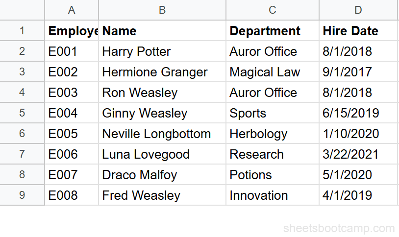
Review your employee data
Open the spreadsheet. Column D has Hire Dates for 8 employees. Harry Potter was hired on 8/1/2018 (a Wednesday), Hermione Granger on 9/1/2017 (a Friday), and Luna Lovegood on 3/22/2021 (a Monday).
Extract the weekday number
Select cell F2 and enter:
=WEEKDAY(D2)For Harry Potter’s hire date of 8/1/2018 (Wednesday), this returns 4 using the default type 1 where Sunday = 1. Copy the formula down to F9.
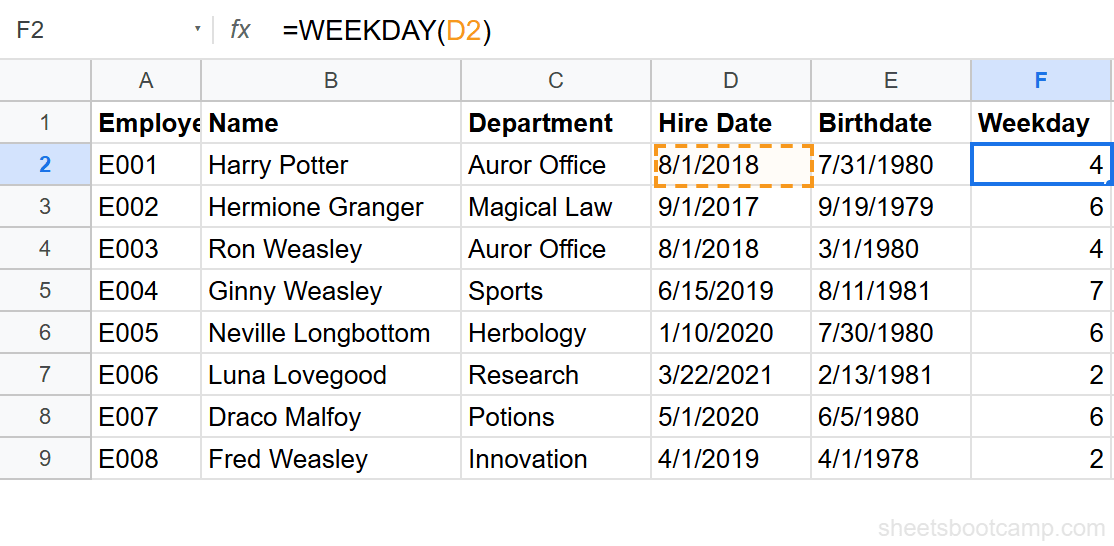
Results for all employees:
- Harry Potter (8/1/2018, Wednesday): 4
- Hermione Granger (9/1/2017, Friday): 6
- Ron Weasley (8/1/2018, Wednesday): 4
- Ginny Weasley (6/15/2019, Saturday): 7
- Neville Longbottom (1/10/2020, Friday): 6
- Luna Lovegood (3/22/2021, Monday): 2
- Draco Malfoy (5/1/2020, Friday): 6
- Fred Weasley (4/1/2019, Monday): 2
Use type 2 for Monday-based numbering
For business applications, type 2 is more intuitive. Change the formula:
=WEEKDAY(D2, 2)For Harry Potter (Wednesday), this returns 3 because Monday = 1. Now weekdays are 1–5 and weekends are 6–7.

Ginny Weasley was hired on 6/15/2019, a Saturday. With type 2, WEEKDAY returns 6 — confirming it’s a weekend. This is useful for flagging entries that shouldn’t have occurred on a non-business day.
Convert to a day name with CHOOSE
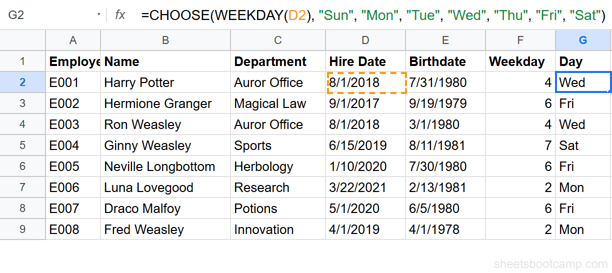
To display the actual day name instead of a number, wrap WEEKDAY in CHOOSE. In cell G2, enter:
=CHOOSE(WEEKDAY(D2), "Sun", "Mon", "Tue", "Wed", "Thu", "Fri", "Sat")For Harry Potter, this returns Wed. For Ginny Weasley, it returns Sat. Copy down to G9 to label all hire dates.
Convert Weekday Numbers to Day Names
There are two approaches to get a day name from a date.
Method 1: CHOOSE + WEEKDAY
=CHOOSE(WEEKDAY(D2), "Sunday", "Monday", "Tuesday", "Wednesday", "Thursday", "Friday", "Saturday")This gives you full control over the output text. Use abbreviated names (“Mon”, “Tue”) or full names (“Monday”, “Tuesday”).
Method 2: TEXT Function
=TEXT(D2, "dddd")This returns the full day name directly. Use "ddd" for three-letter abbreviations: Mon, Tue, Wed. This approach is shorter but less flexible — you cannot customize the output labels.
For more formatting options, see how to format dates in Google Sheets.
Practical Examples
Weekend Detection with IF
Flag each hire date as a weekday or weekend:
=IF(WEEKDAY(D2, 2) > 5, "Weekend", "Weekday")With type 2, values 1–5 are Monday through Friday and 6–7 are Saturday and Sunday. Ginny Weasley (hired Saturday) returns Weekend. All other employees return Weekday.
Highlight Weekends with Conditional Formatting
Apply a custom formula rule to the Hire Date column:
- Select D2:D9
- Go to Format > Conditional formatting
- Set the rule to Custom formula is
- Enter
=WEEKDAY($D2, 2) > 5
Cells with weekend dates get highlighted. The $D2 locks the column but allows the row to change as the rule applies to each row.
Count Hires by Day of Week
Use COUNTIF with WEEKDAY to count how many employees were hired on each day:
=COUNTIF(ARRAYFORMULA(WEEKDAY($D$2:$D$9)), 6)This counts employees hired on a Friday (WEEKDAY = 6 with default type 1). Hermione Granger, Neville Longbottom, and Draco Malfoy were all hired on Fridays, so this returns 3.
Common Errors and How to Fix Them
#VALUE! Error
WEEKDAY returns #VALUE! when the date argument is text instead of a real date.
Fix: Check with =ISNUMBER(D2). If FALSE, the cell contains text. Convert it with =DATEVALUE(D2).
Unexpected Weekday Numbers
You enter =WEEKDAY(D2) and get 4 for what you expected to be Monday. The default type 1 starts with Sunday = 1.
Fix: Add the type argument. Use =WEEKDAY(D2, 2) for Monday = 1 numbering.
#NUM! Error
WEEKDAY returns #NUM! when the type argument is not 1, 2, or 3.
Fix: Use only 1, 2, or 3 as the type argument.
Tips and Best Practices
-
Default to type 2 for business logic. Monday = 1 through Sunday = 7 keeps weekday/weekend checks clean:
WEEKDAY(date, 2) > 5means weekend. -
Use TEXT for quick day names.
=TEXT(D2, "ddd")is shorter than the CHOOSE approach and works for display purposes. Use CHOOSE when you need custom labels. -
Combine with NETWORKDAYS for business day logic. WEEKDAY tells you the day; NETWORKDAYS counts working days. Together they handle schedule-aware formulas.
-
Lock column references in conditional formatting. Use
$D2(notD2) so the column stays fixed while the row adjusts. This prevents the rule from shifting to the wrong column. -
Use WEEKDAY in sorting formulas. To sort a list by day of the week instead of date, add a helper column with
=WEEKDAY(D2, 2)and sort by that column. Monday entries appear first, Sunday entries last.
Related Google Sheets Tutorials
- Google Sheets Date Functions: The Complete Guide — Full reference covering WEEKDAY, NETWORKDAYS, TODAY, and more
- NETWORKDAYS Function — Count business days between dates, excluding weekends and holidays
- TODAY and NOW Functions — Get the current date for live weekday checks
- Conditional Formatting Guide — Highlight weekend dates and apply visual rules to date columns
- IF Function in Google Sheets — Build conditional checks for weekday vs weekend logic
Frequently Asked Questions
What does the WEEKDAY function return in Google Sheets?
WEEKDAY returns a number representing the day of the week for a given date. By default (type 1), Sunday is 1 and Saturday is 7. Use type 2 to make Monday equal 1, or type 3 to make Monday equal 0.
How do I get the day name instead of a number?
Wrap WEEKDAY in CHOOSE to convert the number to a name: =CHOOSE(WEEKDAY(A2), "Sun", "Mon", "Tue", "Wed", "Thu", "Fri", "Sat"). You can also use =TEXT(A2, "dddd") to return the full day name directly without WEEKDAY.
How do I check if a date is a weekend in Google Sheets?
Use =IF(WEEKDAY(A2, 2) > 5, "Weekend", "Weekday"). With type 2, Monday is 1 and Sunday is 7, so values 6 (Saturday) and 7 (Sunday) indicate a weekend.
What are the three type options for WEEKDAY?
Type 1 (default): Sunday = 1, Saturday = 7. Type 2: Monday = 1, Sunday = 7. Type 3: Monday = 0, Sunday = 6. Type 2 is the most common for business applications because it groups weekdays as 1-5 and weekends as 6-7.
Can I use WEEKDAY with conditional formatting?
Yes. Apply a conditional formatting custom formula like =WEEKDAY($D2, 2) > 5 to highlight rows where the date falls on a weekend. This works well for flagging non-business-day entries in a date column.