YEAR, MONTH, and DAY Functions in Google Sheets

YEAR, MONTH, and DAY in Google Sheets extract individual parts from a date. YEAR returns the four-digit year, MONTH returns a number from 1 to 12, and DAY returns the day of the month. These three date functions are the building blocks for grouping data by time period, filtering by month, and reconstructing modified dates.

This guide covers the syntax for all three functions, step-by-step examples using employee hire dates, and practical patterns for counting, grouping, and rebuilding dates.

In This Guide

• Syntax
• How to Use YEAR, MONTH, and DAY: Step-by-Step
• Get Month Names Instead of Numbers
• Practical Examples
• Common Errors and How to Fix Them
• Tips and Best Practices
• Related Google Sheets Tutorials
• Frequently Asked Questions

Syntax

All three functions take a single argument: the date to extract from.

=YEAR(date)

Returns the four-digit year (e.g., 2018).

=MONTH(date)

Returns the month as a number from 1 (January) to 12 (December).

=DAY(date)

Returns the day of the month as a number from 1 to 31.

How to Use YEAR, MONTH, and DAY: Step-by-Step

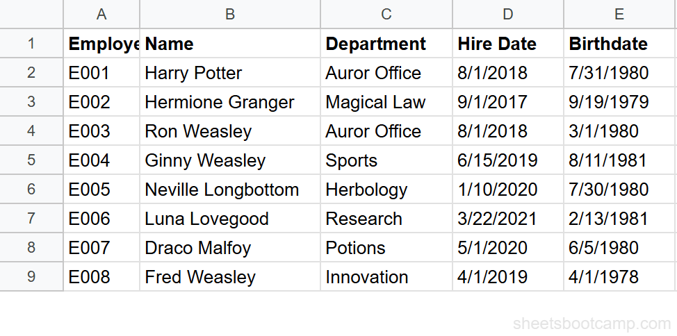
We’ll use the employee database with 8 employees. Column D has Hire Dates and column E has Birthdates.

Sample Data

Open the spreadsheet. Column D contains Hire Dates ranging from 9/1/2017 (Hermione Granger) to 3/22/2021 (Luna Lovegood). Column E contains Birthdates. You’ll extract year, month, and day from the hire dates.

Select cell F2 and enter:

=YEAR(D2)

For Harry Potter’s hire date of 8/1/2018, this returns 2018. Copy the formula down to F9.

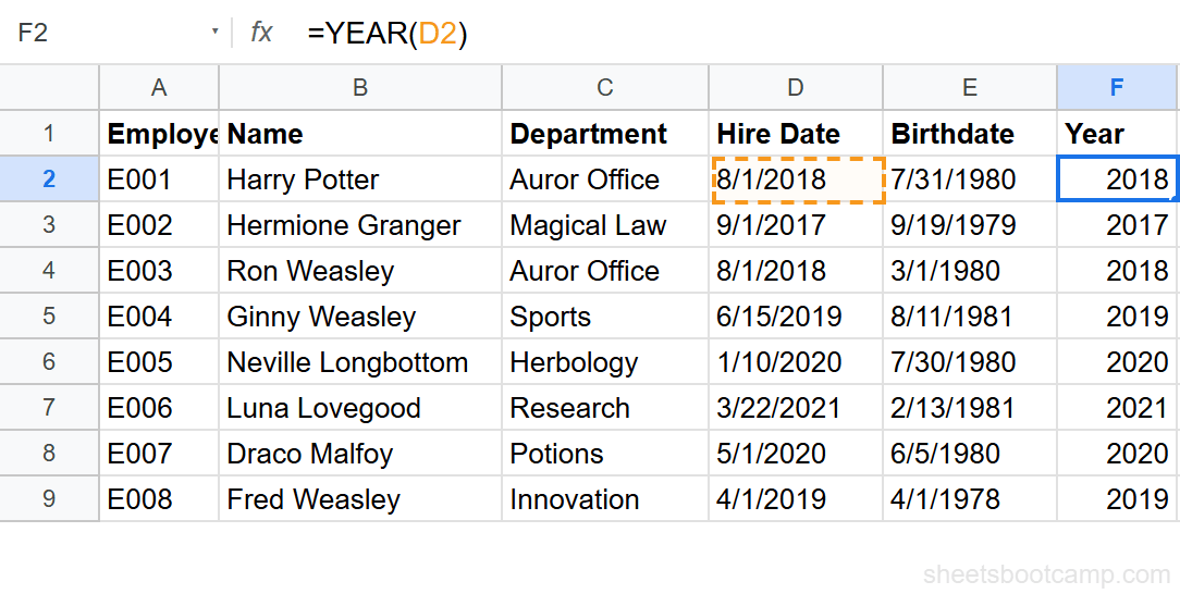
Results across all employees:

• Hermione Granger (9/1/2017): 2017
• Harry Potter, Ron Weasley (8/1/2018): 2018
• Ginny Weasley (6/15/2019), Fred Weasley (4/1/2019): 2019
• Neville Longbottom (1/10/2020), Draco Malfoy (5/1/2020): 2020
• Luna Lovegood (3/22/2021): 2021

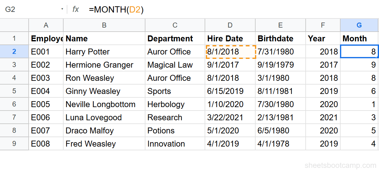
Select cell G2 and enter:

=MONTH(D2)

For Harry Potter (hired 8/1/2018), this returns 8 (August). Copy down to G9. Hermione Granger returns 9, Ginny Weasley returns 6, and Neville Longbottom returns 1.

Select cell H2 and enter:

=DAY(D2)

For Harry Potter (8/1/2018), this returns 1. For Ginny Weasley (6/15/2019), it returns 15. For Luna Lovegood (3/22/2021), it returns 22.

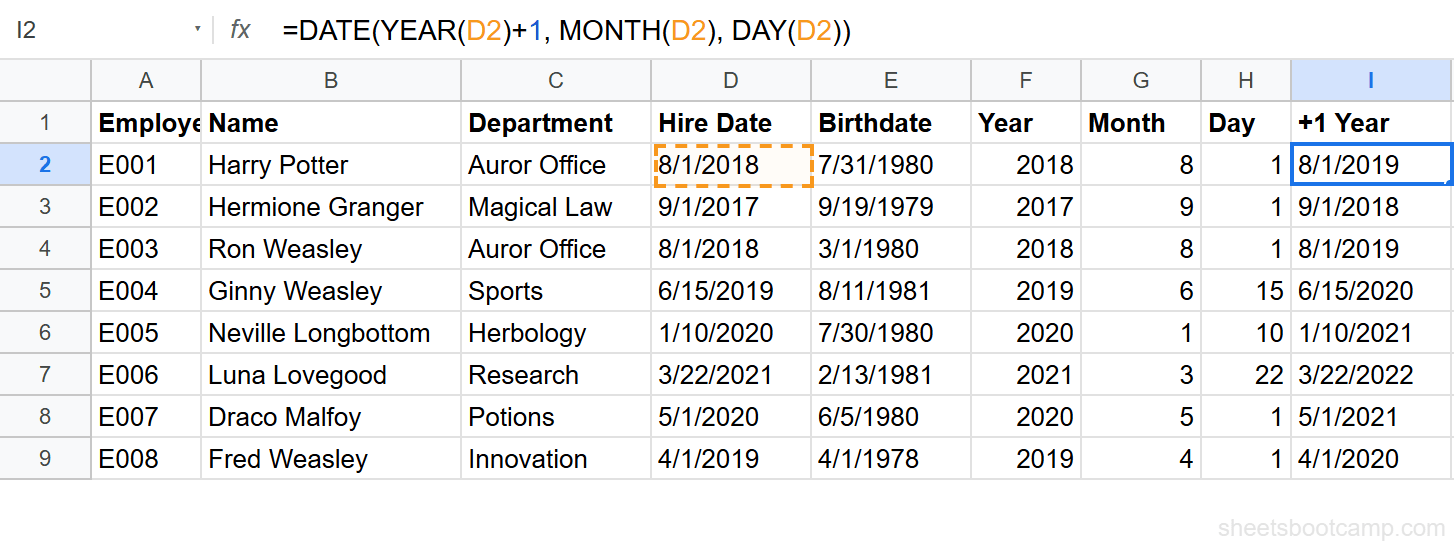
To modify a date, extract its parts, change one, and rebuild with DATE. Select cell I2 and enter:

=DATE(YEAR(D2)+1, MONTH(D2), DAY(D2))

For Harry Potter’s hire date of 8/1/2018, this returns 8/1/2019 — the same date shifted one year forward. The DATE function combines the extracted year (plus 1), original month, and original day into a new date.

For more on adding years to dates, including edge cases with leap years, see the date arithmetic guide.

Get Month Names Instead of Numbers

MONTH returns a number. To display the month name, use TEXT instead:

=TEXT(D2, "MMMM")

For Harry Potter’s hire date (8/1/2018), this returns August. Use "MMM" for the three-letter abbreviation Aug.

For more date formatting options, including custom patterns like “Aug 2018” or “2018-08”, see the formatting guide.

You can also use CHOOSE with MONTH for custom labels:

=CHOOSE(MONTH(D2), "Jan", "Feb", "Mar", "Apr", "May", "Jun", "Jul", "Aug", "Sep", "Oct", "Nov", "Dec")

This gives you full control over the label text.

Practical Examples

Count Hires by Year

Use COUNTIF with ARRAYFORMULA and YEAR to count how many employees were hired each year:

=COUNTIF(ARRAYFORMULA(YEAR($D$2:$D$9)), 2018)

This returns 2 — Harry Potter and Ron Weasley were both hired in 2018. Change 2018 to 2019 and the count becomes 2 (Ginny Weasley and Fred Weasley).

Group by Quarter

Combine MONTH with a formula to assign each hire date to a quarter:

="Q" & INT((MONTH(D2)-1)/3)+1

For Harry Potter (August, month 8): INT((8-1)/3)+1 = INT(2.33)+1 = 3. The result is Q3. For Neville Longbottom (January): Q1. For Fred Weasley (April): Q2.

Build a “Month Year” Label

Combine TEXT with the date to create a sortable label:

=TEXT(D2, "MMM YYYY")

For Harry Potter, this returns Aug 2018. For Hermione Granger, Sep 2017. Use these labels as group headers in reports or pivot-style summaries.

Common Errors and How to Fix Them

#VALUE! Error

YEAR, MONTH, or DAY returns #VALUE! when the cell contains text instead of a real date.

Fix: Check with =ISNUMBER(D2). If FALSE, the value is text. Convert it with =DATEVALUE(D2) before extracting parts.

Result Shows 1899 or 1900

You enter =YEAR(D2) and get 1899. The cell contains a number (like 0 or 1) that Google Sheets interprets as a date near its epoch (12/30/1899).

Fix: Verify that the source cell actually contains a date. If it contains a number from another calculation, YEAR interprets it as a serial date number.

MONTH Returns 1 for All Dates

Every cell returns 1 for MONTH. The column likely contains years (2018, 2019) rather than dates. Google Sheets interprets the number 2018 as the date 7/2/1905, which has a month of 7 — but if you see 1, the values might be even smaller numbers.

Fix: Confirm the source cells are formatted as dates and contain actual date values, not plain numbers.

Tips and Best Practices

1. Use TEXT for display, YEAR/MONTH/DAY for calculations. TEXT returns text strings that look good but cannot be used in math. YEAR, MONTH, and DAY return numbers you can use in formulas.

2. Combine with DATE to modify dates. The pattern =DATE(YEAR(D2)+N, MONTH(D2), DAY(D2)) adds N years. This is the standard way to shift dates by years in Google Sheets.

3. Use MONTH with conditional formatting. Highlight cells where =MONTH($D2) = MONTH(TODAY()) to flag dates in the current month. The rule updates automatically each month because TODAY() changes.

4. ARRAYFORMULA with YEAR enables bulk analysis. =ARRAYFORMULA(YEAR(D2:D9)) returns a column of years. Use this inside COUNTIF, SUMIF, or QUERY to aggregate data by year without helper columns.

5. Watch out for the DATE overflow. =DATE(2026, 13, 1) does not error — it returns 1/1/2027 because month 13 overflows to January of the next year. Google Sheets handles this gracefully, but it can produce unexpected results if your month math goes past 12.

Related Google Sheets Tutorials

• Google Sheets Date Functions: The Complete Guide — Full reference for YEAR, MONTH, DAY, and all date functions
• Add or Subtract Days, Months, Years — Date arithmetic including the DATE function for year shifts
• How to Format Dates — Custom date formats including month names and year-month labels
• TODAY and NOW Functions — Get the current date for live year and month comparisons
• COUNTIF and COUNTIFS — Count dates by year, month, or any other criteria

Frequently Asked Questions

How do I extract the year from a date in Google Sheets?

Use =YEAR(A2) where A2 contains a date. For a date of 8/1/2018, YEAR returns 2018. The result is a four-digit number, not a date.

How do I get the month number from a date in Google Sheets?

Use =MONTH(A2). For 8/1/2018, MONTH returns 8. For 12/25/2026, it returns 12. The result is a number from 1 (January) to 12 (December).

How do I get the month name instead of the month number?

Use =TEXT(A2, "MMMM") for the full month name like August, or =TEXT(A2, "MMM") for the abbreviation like Aug. The TEXT function formats the date directly without needing MONTH.

How do I rebuild a date from separate year, month, and day values?

Use the DATE function: =DATE(year, month, day). For example, =DATE(YEAR(A2)+1, MONTH(A2), DAY(A2)) adds one year to the date in A2 by extracting each part, modifying the year, and reconstructing the date.

Can I use YEAR and MONTH with COUNTIF?

Yes. Use COUNTIF with ARRAYFORMULA to count dates by year or month. =COUNTIF(ARRAYFORMULA(YEAR(D2:D9)), 2018) counts how many dates in D2:D9 fall in 2018. For Harry Potter and Ron Weasley (both hired 8/1/2018), the count is 2.