IF with AND and OR in Google Sheets
Learn how to use IF with AND and OR in Google Sheets to test multiple conditions. Step-by-step examples for combining logical functions in one formula.
Sheets Bootcamp
February 25, 2026
IF with AND and OR in Google Sheets lets you test multiple conditions in a single formula. The basic IF function checks one condition. AND and OR extend it so you can check two, three, or more conditions at once. We’ll cover both functions with step-by-step examples, then show you how to combine them.
In This Guide
- How AND Works
- How OR Works
- Sample Data
- IF with AND: Step-by-Step
- IF with OR: Step-by-Step
- Combining AND and OR in One Formula
- Multiple AND Conditions
- Common Mistakes
- Tips
- Related Google Sheets Tutorials
- FAQ
How AND Works
AND returns TRUE only when every condition inside it is TRUE. If any single condition is FALSE, AND returns FALSE.
=AND(condition1, condition2, condition3, ...)You can include up to 30 conditions. Every one of them must be TRUE for AND to return TRUE. For example, =AND(10>5, 3<7) returns TRUE because both comparisons are true. Change either one to a false comparison and AND returns FALSE.
How OR Works
OR returns TRUE when at least one condition inside it is TRUE. OR only returns FALSE when every condition is FALSE.
=OR(condition1, condition2, condition3, ...)For example, =OR(10>5, 3>7) returns TRUE because the first comparison is true, even though the second is false. OR is useful when meeting any one of several criteria is enough to trigger an action.
AND and OR by themselves return only TRUE or FALSE. To get a custom result like “Priority” or “Standard”, nest AND or OR inside an IF formula as the logical test.
Sample Data
We’ll use a sales records table with 10 rows of data in columns A through G.
| Date | Salesperson | Region | Product | Units | Revenue | Commission |
|---|---|---|---|---|---|---|
| 1/5/2026 | Fred Weasley | Diagon Alley | Extendable Ears | 12 | $239.88 | $24.00 |
| 1/7/2026 | Ginny Weasley | Hogsmeade | Self-Stirring Cauldron | 8 | $360.00 | $36.00 |
| 1/8/2026 | Lee Jordan | Diagon Alley | Remembrall | 15 | $525.00 | $52.50 |
| 1/10/2026 | Fred Weasley | Diagon Alley | Omnioculars | 5 | $325.00 | $32.50 |
| 1/12/2026 | George Weasley | Hogsmeade | Sneakoscope | 20 | $570.00 | $57.00 |
| 1/14/2026 | Ginny Weasley | Hogwarts | Nimbus 2000 | 25 | $624.75 | $62.50 |
| 1/15/2026 | Lee Jordan | Hogsmeade | Extendable Ears | 10 | $199.90 | $20.00 |
| 1/18/2026 | Fred Weasley | Diagon Alley | Invisibility Cloak | 3 | $269.97 | $27.00 |
| 1/20/2026 | George Weasley | Hogwarts | Firebolt | 8 | $336.00 | $33.60 |
| 1/22/2026 | Ginny Weasley | Hogsmeade | Deluminator | 6 | $330.00 | $33.00 |
IF with AND: Step-by-Step
We want to label each sale as “Priority” when the region is Diagon Alley and the revenue exceeds $300. Both conditions must be true.
Step 1: Review Your Conditions
The two conditions are:
- Column C (Region) equals “Diagon Alley”
- Column F (Revenue) is greater than $300
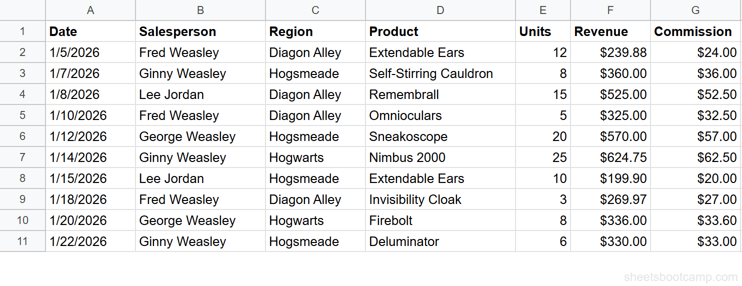
If you tested =AND(C2="Diagon Alley", F2>300) by itself in a cell, it would return TRUE or FALSE. We’ll wrap this in IF to get a label instead.
Step 2: Enter the IF + AND Formula
Select cell H1 and enter the header Status. Then select cell H2 and enter:
=IF(AND(C2="Diagon Alley", F2>300), "Priority", "Standard")This checks both conditions. If C2 is “Diagon Alley” and F2 is greater than 300, the cell returns “Priority”. If either condition fails, it returns “Standard”.
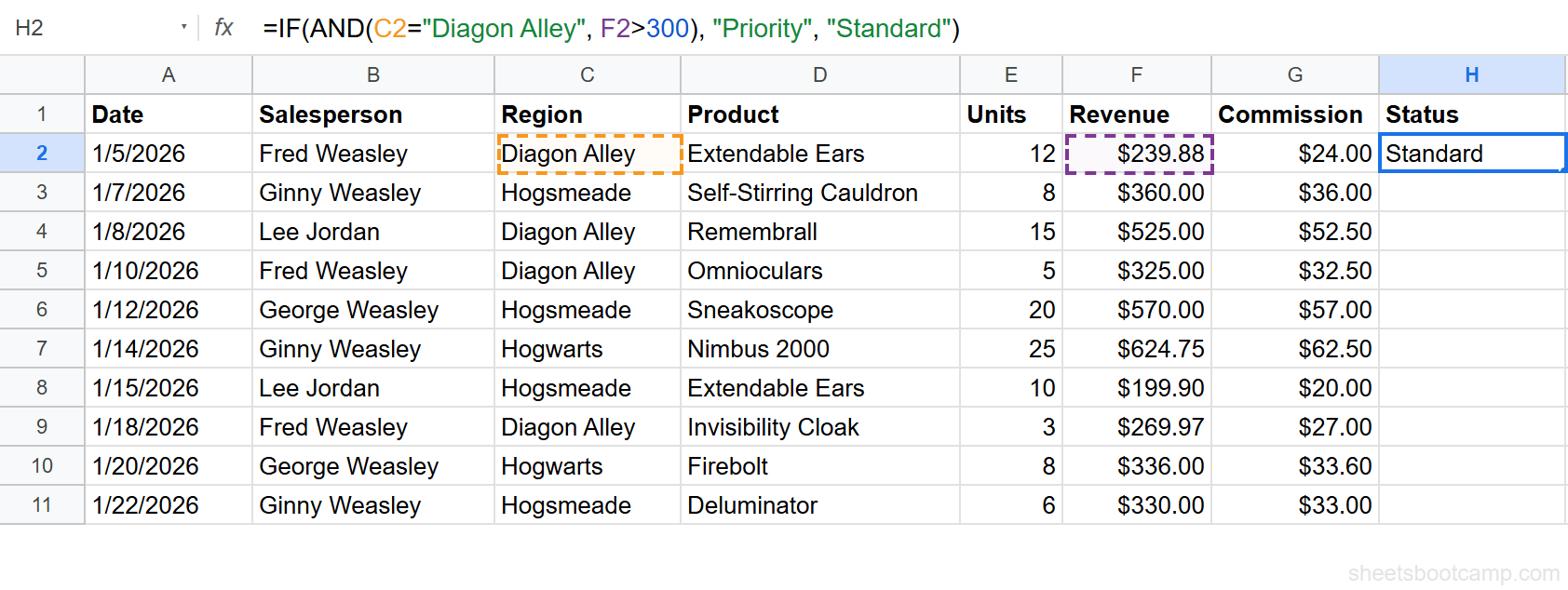
Step 3: Copy Down and Review Results
Copy the formula from H2 down through H11. Two rows return “Priority”:
- Row 3 (Lee Jordan, Diagon Alley, $525.00) — both conditions met
- Row 4 (Fred Weasley, Diagon Alley, $325.00) — both conditions met
The remaining eight rows return “Standard”. Row 1 (Fred Weasley, Diagon Alley, $239.88) fails because the revenue is under $300. Rows in Hogsmeade or Hogwarts fail the region check regardless of revenue.
IF with OR: Step-by-Step
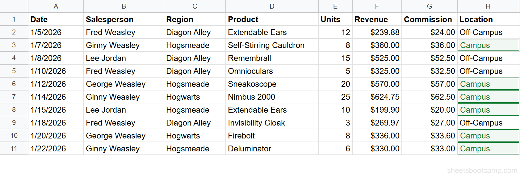
Now we want to label each sale as “Campus” when the region is Hogwarts or Hogsmeade. Either condition is enough.
Step 1: Enter the IF + OR Formula
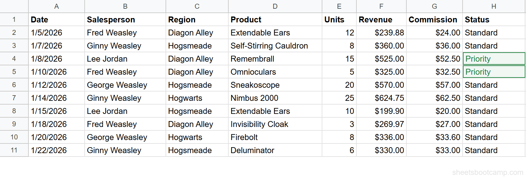
Clear column H or use column I. In H2 (with “Location” as the header in H1), enter:
=IF(OR(C2="Hogwarts", C2="Hogsmeade"), "Campus", "Off-Campus")This checks whether C2 matches either region. If at least one comparison is true, the formula returns “Campus”. If neither matches (meaning the region is Diagon Alley), it returns “Off-Campus”.
Step 2: Copy Down and Review Results
Copy H2 down through H11. Six rows return “Campus”:
- Row 2 (Hogsmeade), Row 5 (Hogsmeade), Row 6 (Hogwarts), Row 7 (Hogsmeade), Row 9 (Hogwarts), Row 10 (Hogsmeade)
The four Diagon Alley rows (1, 3, 4, 8) return “Off-Campus”.
OR works well when you have a short list of values to check. If you have more than three or four values, consider using REGEXMATCH or MATCH instead for cleaner formulas: =IF(MATCH(C2, {"Hogwarts","Hogsmeade"}, 0), "Campus", "Off-Campus").
Combining AND and OR in One Formula
You can nest AND inside OR (or OR inside AND) to build more precise conditions. Here we want to label a sale as “Bonus” when either of these groups is true:
- Diagon Alley and revenue over $300
- Hogwarts and units over 10
=IF(OR(AND(C2="Diagon Alley", F2>300), AND(C2="Hogwarts", E2>10)), "Bonus", "Standard")The OR function wraps two AND functions. If either AND group returns TRUE, the IF formula returns “Bonus”. Three rows qualify:
- Row 3 (Diagon Alley, $525.00) — first AND group
- Row 4 (Diagon Alley, $325.00) — first AND group
- Row 6 (Hogwarts, 25 units) — second AND group
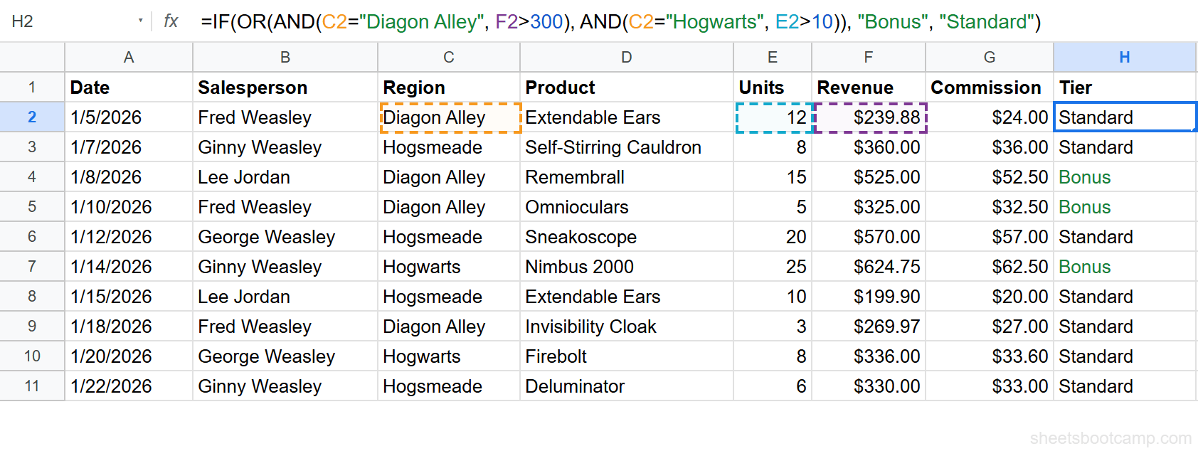
Row 9 (Hogwarts, 8 units) does not qualify because 8 is not greater than 10.
Multiple AND Conditions
AND accepts more than two conditions. Here we add a third: Diagon Alley, revenue over $300, and units over 10.
=IF(AND(C2="Diagon Alley", F2>300, E2>10), "Top Performer", "Standard")Only Row 3 (Lee Jordan, Diagon Alley, $525.00, 15 units) meets all three conditions. Row 4 (Fred Weasley, Diagon Alley, $325.00, 5 units) fails the units check.
Each new condition narrows the result further. AND with three conditions is stricter than AND with two.
Common Mistakes
Putting Conditions as Separate IF Arguments
A common error is writing conditions as separate arguments to IF instead of wrapping them in AND or OR.
Wrong:
=IF(C2="Diagon Alley", F2>300, "Standard")This looks like two conditions, but Google Sheets reads three arguments: the logical test is C2="Diagon Alley", the value_if_true is F2>300 (which returns TRUE or FALSE), and the value_if_false is “Standard”. When C2 is “Diagon Alley”, you get TRUE or FALSE instead of “Priority”.
Correct:
=IF(AND(C2="Diagon Alley", F2>300), "Priority", "Standard")Always wrap multiple conditions inside AND() or OR() before passing them to IF.
IF takes exactly three arguments: logical_test, value_if_true, value_if_false. You cannot add extra conditions by adding more arguments. Use AND or OR to combine conditions into a single logical test.
Confusing AND with OR
AND means “all must be true.” OR means “any can be true.” Mixing them up produces the wrong results with no error message. Before writing a formula, state the rule in plain language: “I need both conditions” means AND. “I need at least one” means OR.
Missing Commas Between Conditions
Forgetting the comma between conditions inside AND or OR produces a formula parse error. Each condition must be separated by a comma:
=AND(C2="Diagon Alley" F2>300) — missing comma, formula breaks.
=AND(C2="Diagon Alley", F2>300) — correct.
Tips
-
Test AND/OR standalone first. Before nesting inside IF, enter
=AND(C2="Diagon Alley", F2>300)in a blank cell. Confirm it returns TRUE or FALSE as expected. Then wrap it in IF. This makes debugging faster. -
Use ARRAYFORMULA for column-wide application. Instead of copying the formula down, wrap it in ARRAYFORMULA:
=ARRAYFORMULA(IF(AND(C2:C11="Diagon Alley", F2:F11>300), "Priority", "Standard")). This fills the entire column with one formula. -
Apply AND/OR logic visually. Conditional formatting formula-based rules use the same AND/OR syntax. You can highlight Diagon Alley rows with revenue over $300 using
=AND(C2="Diagon Alley", F2>300)as a custom formula rule. -
QUERY WHERE uses similar logic. If you work with large datasets, QUERY supports WHERE clauses with AND and OR operators. The syntax is different, but the logic is the same.
Related Google Sheets Tutorials
- IF Function in Google Sheets: Complete Guide - Full syntax breakdown, nested IF, and all logical operators
- Nested IF in Google Sheets - Build decision trees with multiple IF levels and combine with AND/OR
- IFS Function in Google Sheets - Check multiple conditions without nesting when each condition has a unique result
- Conditional Formatting in Google Sheets - Apply AND/OR logic visually with formula-based formatting rules
- QUERY Function in Google Sheets - Filter data with AND/OR conditions using SQL-like WHERE clauses
FAQ
How do you use IF with AND in Google Sheets?
Nest AND inside IF as the logical test. The syntax is =IF(AND(condition1, condition2), value_if_true, value_if_false). AND returns TRUE only when every condition is met, so IF returns the true value only when all conditions pass.
How do you use IF with OR in Google Sheets?
Nest OR inside IF as the logical test. The syntax is =IF(OR(condition1, condition2), value_if_true, value_if_false). OR returns TRUE when at least one condition is met, so IF returns the true value when any condition passes.
Can you combine AND and OR in one IF formula?
Yes. Place AND and OR together inside the IF logical test using the structure =IF(OR(AND(cond1, cond2), AND(cond3, cond4)), value_if_true, value_if_false). This checks whether either group of conditions is met.
What is the difference between AND and OR in Google Sheets?
AND returns TRUE only when all conditions are TRUE. OR returns TRUE when at least one condition is TRUE. Use AND when every condition must be met. Use OR when meeting any one condition is enough.