IFERROR in Google Sheets: Hide Errors Gracefully
Learn how to use IFERROR in Google Sheets to replace formula errors with custom messages or blanks. Step-by-step examples with VLOOKUP and INDEX MATCH.
Sheets Bootcamp
May 21, 2026
The IFERROR function in Google Sheets catches formula errors and replaces them with a value you choose. Errors like #N/A, #DIV/0!, and #REF! break the look of your spreadsheet and can cause problems in downstream calculations. IFERROR wraps around any formula and returns a clean result when something goes wrong. As part of the IF functions family, it is one of the most practical error-handling tools in Sheets. We will cover the syntax, walk through a VLOOKUP example step-by-step, and show how IFERROR works with division and INDEX MATCH.
In This Guide
- IFERROR Syntax and Parameters
- How to Use IFERROR with VLOOKUP: Step-by-Step
- IFERROR Examples
- Common Errors and Mistakes
- Tips and Best Practices
- Related Google Sheets Tutorials
- FAQ
IFERROR Syntax and Parameters
Here is the IFERROR formula structure in Google Sheets:
=IFERROR(value, [value_if_error])IFERROR takes two arguments. The first is the formula to evaluate. The second is what to return if that formula produces an error.
| Parameter | Description | Required |
|---|---|---|
| value | The formula or expression to evaluate. This can be any formula, cell reference, or calculation. | Yes |
| value_if_error | The value returned when the first argument produces an error. Can be text, a number, a blank string, or another formula. Defaults to an empty value if omitted. | No |
Google Sheets evaluates the first argument. If it returns a valid result, IFERROR passes that result through unchanged. If it returns any error (#N/A, #DIV/0!, #REF!, #VALUE!, #NAME?, #NUM!, or #NULL!), IFERROR returns the second argument instead.
IFERROR catches every error type. This means it can hide errors that signal real problems in your formula. If you only want to catch #N/A from a failed lookup, use IFNA instead. That way, errors like #REF! (deleted column) or #VALUE! (wrong data type) still appear and alert you to fix them.
How to Use IFERROR with VLOOKUP: Step-by-Step
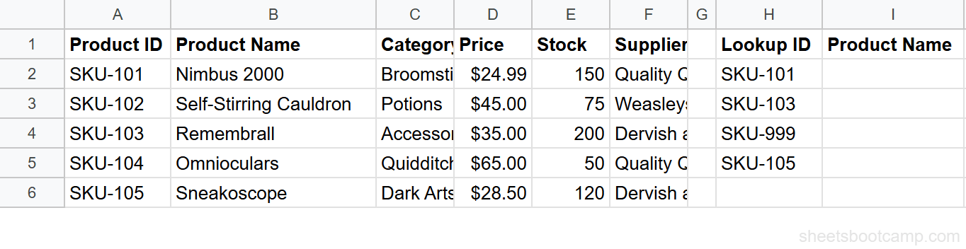
We will use the product inventory table with 8 rows. The goal: look up product names by ID and show “Not found” instead of #N/A when an ID does not exist.
Set up a lookup column
Your spreadsheet has product data in columns A through F. Column A contains Product ID and column B contains Product Name. In cell H1, type the header “Lookup ID”. In cells H2 through H5, enter these product IDs:
- H2: SKU-101
- H3: SKU-103
- H4: SKU-999 (this ID does not exist)
- H5: SKU-105
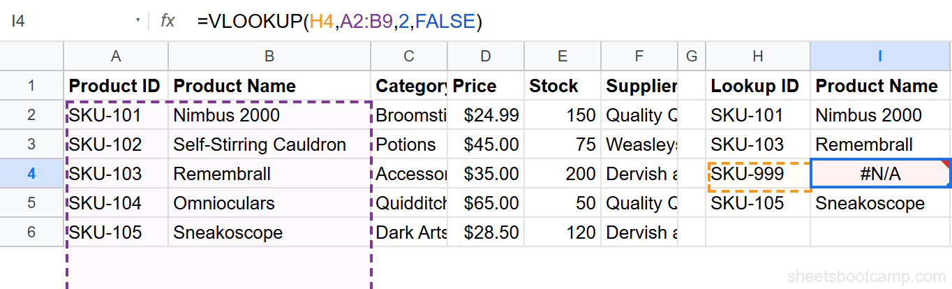
Enter a VLOOKUP without IFERROR
Select cell I2 and enter this formula:
=VLOOKUP(H2,A2:B9,2,FALSE)This searches column A for the value in H2 and returns the matching Product Name from column B. For SKU-101, it returns “Nimbus 2000”. Copy the formula down to I5. Cell I4 shows #N/A because SKU-999 does not exist in your product table.
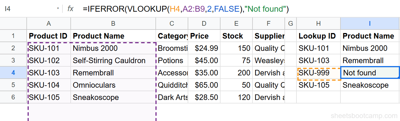
Wrap VLOOKUP in IFERROR
Edit cell I2 and change the formula to:
=IFERROR(VLOOKUP(H2,A2:B9,2,FALSE),"Not found")Copy down to I5. Here are the results:
- I2: Nimbus 2000 (SKU-101 found)
- I3: Remembrall (SKU-103 found)
- I4: Not found (SKU-999 does not exist)
- I5: Sneakoscope (SKU-105 found)
The three valid lookups return the correct product names. The missing ID returns “Not found” instead of #N/A.
Use "Not found" or "N/A" as your fallback text when building reports. Avoid leaving the second argument empty in shared sheets. A blank cell looks like missing data, and other people will not know whether the formula ran or the value was never entered.
IFERROR Examples
Example 1: IFERROR with Division
Division by zero returns #DIV/0! in Google Sheets. This happens when you calculate averages, rates, or percentages and a denominator cell is empty or zero.
=IFERROR(E2/F2,0)If F2 contains 0, this returns 0 instead of #DIV/0!. If F2 contains a valid number like 5, the formula returns the division result normally. Using 0 as the fallback keeps your column numeric so SUM and AVERAGE functions still work on the output range.
Example 2: IFERROR with INDEX MATCH
INDEX MATCH returns #N/A when the MATCH function cannot find the lookup value. IFERROR handles this the same way it handles VLOOKUP errors.
=IFERROR(INDEX(B2:B9,MATCH(H2,A2:A9,0)),"Not found")This searches column A for the value in H2 and returns the matching value from column B. For SKU-103, it returns “Remembrall”. For SKU-999, it returns “Not found”. The formula works identically to the IFERROR VLOOKUP example, but INDEX MATCH can search any column, not only the leftmost one.
Example 3: Nested IFERROR for Multiple Lookups
You can nest IFERROR to search multiple ranges. If the first lookup fails, try a second range before returning a fallback.
=IFERROR(VLOOKUP(H2,A2:B9,2,FALSE),IFERROR(VLOOKUP(H2,K2:L9,2,FALSE),"Not in either table"))This searches the product inventory first. If the ID is not found, it searches a second table in columns K through L. If both lookups fail, it returns “Not in either table”. This pattern is useful when your data is split across multiple sheets or ranges.
Common Errors and Mistakes
Wrapping Too Much in IFERROR
IFERROR catches all errors, including ones that indicate real formula problems. If your VLOOKUP has a #REF! error because you deleted a column, IFERROR hides that too. You will not know the formula is broken.
The fix: Use IFNA instead of IFERROR when you only need to handle missing lookup values. IFNA catches #N/A and lets #REF!, #VALUE!, and other errors show.
=IFNA(VLOOKUP(H2,A2:B9,2,FALSE),"Not found")Putting IFERROR Inside the Formula
A common mistake is placing IFERROR around only part of the formula instead of the entire expression.
Wrong:
=VLOOKUP(IFERROR(H2,A2:B9,2,FALSE))Correct:
=IFERROR(VLOOKUP(H2,A2:B9,2,FALSE),"Not found")IFERROR must wrap the formula that produces the error. Placing it inside the VLOOKUP changes the meaning of the arguments and returns a #VALUE! or #ERROR! result.
Using IFERROR to Mask Data Problems
If every row in a lookup returns “Not found”, the issue is not the formula. Your lookup values likely have trailing spaces, different formatting, or mismatched data types. IFERROR hides the symptom. Fix the source data first using TRIM or VALUE, then add IFERROR for genuine edge cases.
If your IFERROR fallback triggers on most rows, remove the IFERROR temporarily and investigate the raw errors. Widespread #N/A results usually mean a data mismatch, not a missing record. Fix the root cause before wrapping in IFERROR.
Tips and Best Practices
-
Use IFNA for lookups, IFERROR for everything else. IFNA catches only #N/A, which is the expected error when a lookup value is missing. IFERROR catches all errors, which can hide formula bugs. Reserve IFERROR for division, calculations, and cases where multiple error types are expected.
-
Return a consistent data type. If your formula returns numbers, use a number as the fallback (like 0), not text. Mixing numbers and text in a column breaks SUM, AVERAGE, and chart data ranges.
-
Return a blank string for clean reports. Use
=IFERROR(formula,"")when you want error cells to appear empty. This is useful for printed reports and dashboards where “Not found” text would clutter the layout. -
Combine with nested IF for conditional error handling. You can use IF inside the fallback argument:
=IFERROR(VLOOKUP(H2,A2:B9,2,FALSE),IF(H2="","Enter an ID","Not found")). This returns different messages depending on whether the lookup cell is empty or the value genuinely does not exist. -
Test your formula without IFERROR first. Write and verify the core formula before wrapping it. Add IFERROR as the last step once you have confirmed the formula works on valid data. This prevents IFERROR from hiding mistakes you made while building the formula.
Google Sheets also has an ISERROR function that returns TRUE or FALSE instead of replacing the error. Use ISERROR inside IF statements for custom logic: =IF(ISERROR(A1/B1),"Cannot calculate",A1/B1). IFERROR is shorter for most cases.
Related Google Sheets Tutorials
- IF Statements in Google Sheets - Learn the core IF function and other conditional formulas
- VLOOKUP Errors and How to Fix Them - Troubleshoot #N/A, #REF!, and #VALUE! errors in VLOOKUP
- INDEX MATCH in Google Sheets - A more flexible alternative to VLOOKUP for looking up data
- Nested IF Statements - Build multi-tier conditions when a single IF is not enough
- IFS Function - Evaluate multiple conditions in a flat formula without nesting
Frequently Asked Questions
What does IFERROR do in Google Sheets?
IFERROR checks whether a formula returns an error. If it does, IFERROR returns a value you specify instead of the error. If the formula works normally, IFERROR returns the original result unchanged.
How do I use IFERROR with VLOOKUP?
Wrap the entire VLOOKUP inside IFERROR. For example, =IFERROR(VLOOKUP("SKU-999",A2:D5,2,FALSE),"Not found") returns the text “Not found” instead of #N/A when the lookup value does not exist in your range.
Can IFERROR return a blank cell instead of an error?
Yes. Use an empty string as the second argument. For example, =IFERROR(A1/B1,"") returns a blank cell when B1 is zero, instead of showing #DIV/0!.
What is the difference between IFERROR and IFNA?
IFERROR catches all error types including #N/A, #DIV/0!, #REF!, #VALUE!, and #NAME?. IFNA catches only #N/A errors and lets other error types show. Use IFNA when you want to handle missing lookups but still see other errors that indicate real formula problems.
Does IFERROR slow down Google Sheets?
IFERROR adds minimal overhead. Google Sheets evaluates the formula inside IFERROR first. If it succeeds, the IFERROR wrapper has almost no performance cost. On large sheets with thousands of rows, the lookup or calculation inside IFERROR is what affects speed, not IFERROR itself.