IFS Function in Google Sheets (With Examples)
Learn how to use the IFS function in Google Sheets to evaluate multiple conditions without nesting. Includes real examples, IFS vs nested IF, and tips.
Sheets Bootcamp
February 24, 2026
The IFS function in Google Sheets evaluates multiple conditions in order and returns a value for the first one that is TRUE. If you have been writing nested IF statements to handle three or more outcomes, IFS gives you the same result in a flat, readable formula. We’ll cover the syntax, walk through a revenue classification example, compare IFS to nested IF side-by-side, and flag the mistakes that trip most people up.
In This Guide
- IFS Syntax and Parameters
- How to Classify Revenue with IFS: Step-by-Step
- IFS vs Nested IF
- IFS Examples
- Common Mistakes
- Tips and Best Practices
- Related Google Sheets Tutorials
- FAQ
IFS Syntax and Parameters
Here is the IFS formula structure in Google Sheets:
=IFS(condition1, value1, condition2, value2, ...)IFS takes pairs of arguments. Each pair is a condition followed by the value to return if that condition is TRUE.
| Parameter | Description | Required |
|---|---|---|
| condition1 | The first logical test to evaluate | Yes |
| value1 | The value returned if condition1 is TRUE | Yes |
| condition2 | The second logical test, evaluated only if condition1 is FALSE | Yes |
| value2 | The value returned if condition2 is TRUE | Yes |
| … | Additional condition/value pairs as needed | No |
Google Sheets evaluates conditions from left to right. It stops at the first TRUE condition and returns that pair’s value. Every condition after the first match is ignored.
IFS has no built-in default value. If none of your conditions are TRUE, the formula returns #N/A. Always add TRUE as your last condition to act as a catchall. For example: =IFS(A1>=90,"A", A1>=80,"B", TRUE,"C").
How to Classify Revenue with IFS: Step-by-Step
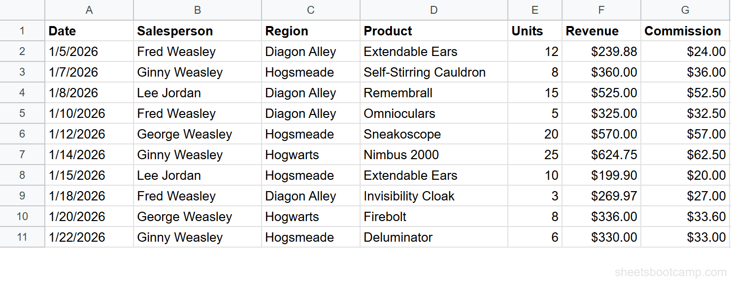
We’ll use a sales records table with 10 rows. The goal: classify each sale’s revenue as “High” ($500+), “Medium” ($300-$499), or “Low” (under $300).
Review your data
Your spreadsheet has sales data in columns A through G. Column F contains Revenue. You will add the IFS formula in column H.
Enter the IFS formula
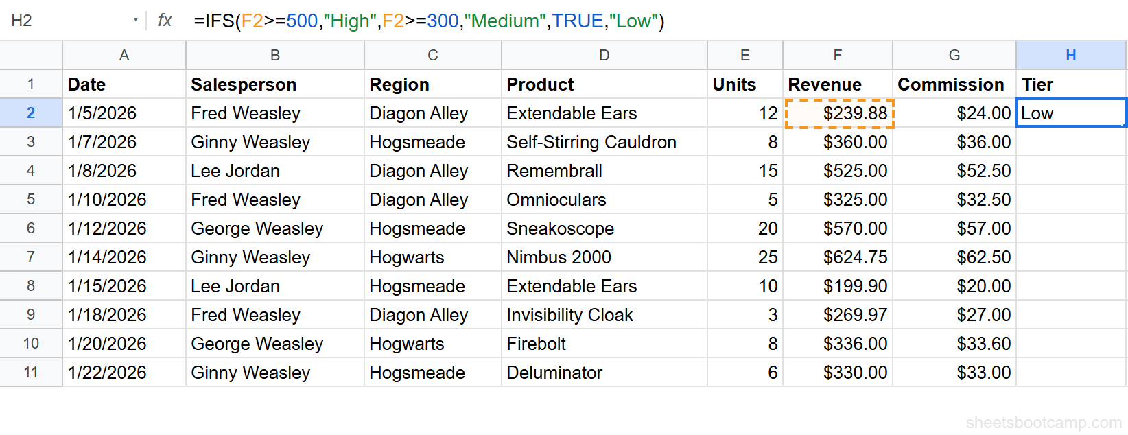
Select cell H2 and enter this formula:
=IFS(F2>=500,"High",F2>=300,"Medium",TRUE,"Low")This tests three conditions in order:
- Is F2 greater than or equal to 500? If yes, return “High”.
- Is F2 greater than or equal to 300? If yes, return “Medium”.
- TRUE (always matches). Return “Low”.
F2 contains $239.88, which fails the first two tests. The TRUE catchall returns “Low”.
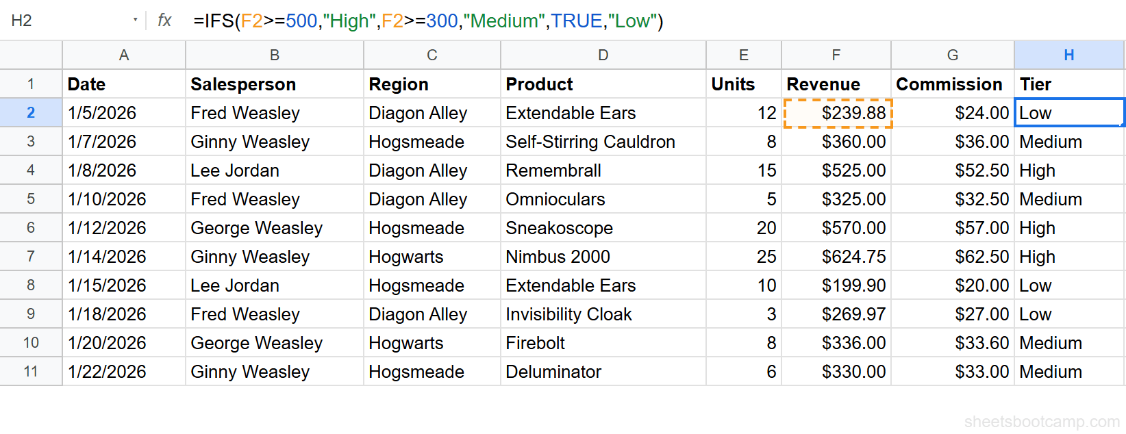
Review the results and fill down
Drag the fill handle from H2 down to H11 to classify all 10 rows. Here are the results:
- $239.88 returns “Low”
- $360.00 returns “Medium”
- $525.00 returns “High”
- $325.00 returns “Medium”
- $570.00 returns “High”
- $624.75 returns “High”
- $199.90 returns “Low”
- $269.97 returns “Low”
- $336.00 returns “Medium”
- $330.00 returns “Medium”
You can also type the formula in H2 and press Ctrl+Enter to stay in the cell, then double-click the fill handle to auto-fill down to the last row of data.
IFS vs Nested IF
Here is the same revenue classification written both ways.
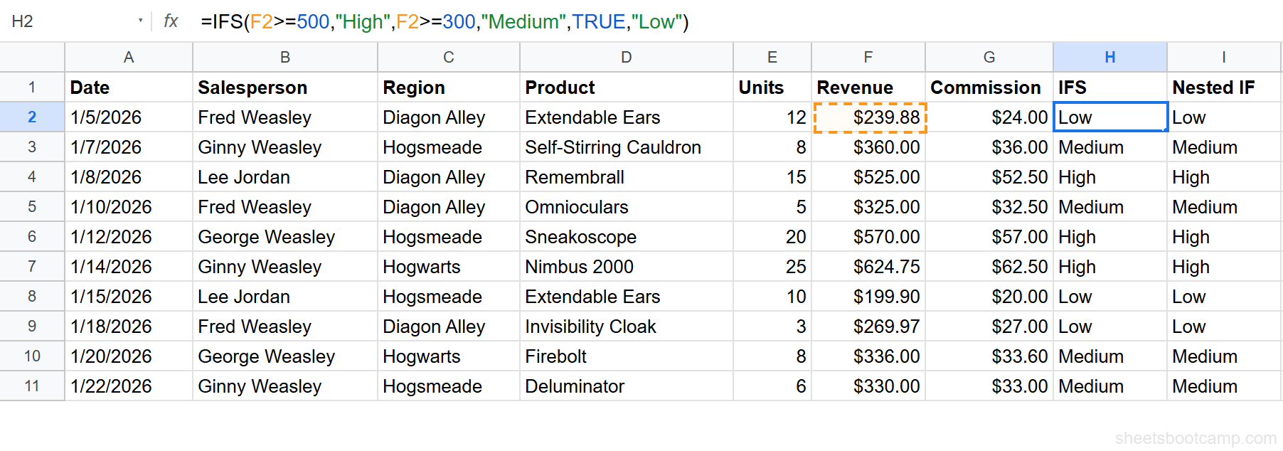
IFS version:
=IFS(F2>=500,"High",F2>=300,"Medium",TRUE,"Low")Nested IF version:
=IF(F2>=500,"High",IF(F2>=300,"Medium","Low"))Both formulas return the same results. For three tiers, the difference is small. But add more conditions and the gap widens fast.
With five tiers, IFS stays flat:
=IFS(F2>=1000,"Elite",F2>=500,"High",F2>=300,"Medium",F2>=100,"Low",TRUE,"Minimal")The nested IF version for five tiers requires four levels of nesting, four closing parentheses, and careful counting to figure out which IF belongs to which condition. IFS reads top-to-bottom like a checklist.
When nested IF still makes sense: If you have two outcomes (yes/no, pass/fail), a regular IF statement is cleaner. IFS is not worth it for a single condition.
IFS Examples
Example 1: Letter Grades Based on Units Sold
You want to grade salesperson performance by units sold in column E.
=IFS(E2>=20,"A",E2>=10,"B",E2>=5,"C",TRUE,"D")For row 1 (12 units), this returns “B”. For row 5 (20 units), this returns “A”. For row 4 (5 units), this returns “C”. For row 9 (8 units), this returns “C”. The conditions test from highest to lowest, and the TRUE catchall assigns “D” to anyone with fewer than 5 units.
Example 2: Commission Rate Tiers
Instead of returning text, IFS can return a calculation. Here, the commission rate depends on revenue:
=IFS(F2>=500,F2*0.12,F2>=300,F2*0.10,TRUE,F2*0.08)For row 3 ($525.00 revenue), this returns $63.00 (12% rate). For row 2 ($360.00), this returns $36.00 (10% rate). For row 1 ($239.88), this returns $19.19 (8% rate). Each value slot runs a different calculation based on which tier matched.
Common Mistakes
Testing Conditions in the Wrong Order
IFS stops at the first TRUE condition. If you test the smallest value first, every row matches it.
=IFS(F2>=100,"Low",F2>=300,"Medium",F2>=500,"High")This formula returns “Low” for every row because all revenue values are above $100. The F2>=300 and F2>=500 conditions never get evaluated. Always test from largest to smallest.
Condition order in IFS determines results. Test the most restrictive condition first (highest threshold), then work down. If you reverse the order, every row matches the first condition and IFS stops checking.
Forgetting the TRUE Catchall
If no condition matches, IFS returns #N/A. This catches people off guard because IF has a built-in else clause.
=IFS(F2>=500,"High",F2>=300,"Medium")Any revenue under $300 returns #N/A with this formula. Add TRUE,"Low" as the last pair to handle remaining cases.
Using IFS for Two Conditions
If you only have two outcomes, a regular IF is shorter and clearer:
=IF(F2>=500,"High","Not High")IFS adds value when you have three or more condition/value pairs. For a binary choice, stick with IF.
Tips and Best Practices
-
Always end with a TRUE catchall. This is the IFS equivalent of the “else” in a regular IF statement. Without it, unexpected values return #N/A.
-
Order conditions from most restrictive to least. Test >=500 before >=300 before TRUE. The first match wins.
-
Use IFS for three or more tiers. For two outcomes, IF is better. For three or more, IFS is easier to read and edit.
-
Combine IFS with AND or OR for multi-column conditions. For example,
=IFS(AND(E2>=20,F2>=500),"Star",E2>=10,"Solid",TRUE,"Developing")tests both units and revenue for the top tier. -
Add a header label in column H. Label it “Tier” or “Grade” so the classification column is clear to anyone reading your sheet.
IFS is available in Google Sheets and Excel 2019+. If you share files with users on older Excel versions, they will see a compatibility error. In that case, use nested IF instead.
Related Google Sheets Tutorials
- IF Statements in Google Sheets - Learn the foundational IF function that IFS builds on
- Nested IF Statements - When you need the nested approach instead of IFS
- IF with AND, OR, NOT - Combine logical operators with IF and IFS for multi-condition tests
- QUERY Function - Filter and classify data using SQL-like syntax as an alternative to formula-based approaches
Frequently Asked Questions
What is the IFS function in Google Sheets?
IFS evaluates multiple conditions in order and returns the value for the first condition that is TRUE. It works like a series of IF statements written in a flat list instead of nested inside each other.
What is the difference between IF and IFS?
IF tests one condition and has a built-in else clause. IFS tests multiple conditions in sequence with no built-in default. For two outcomes, use IF. For three or more, IFS is easier to read and maintain.
How do I add a default value to IFS?
Add TRUE as the last condition with your default value. For example, =IFS(A1>=500,"High",A1>=300,"Medium",TRUE,"Low"). The TRUE condition always matches, so it catches everything the earlier conditions missed.
Can IFS return calculations instead of text?
Yes. Each value in IFS can be a formula, cell reference, or calculation. For example, =IFS(F2>=500,F2*0.12,F2>=300,F2*0.10,TRUE,F2*0.08) returns a calculated commission amount based on revenue tiers.