IMPORTRANGE in Google Sheets: Complete Guide
Learn how to use IMPORTRANGE in Google Sheets to pull data from other spreadsheets. Covers syntax, access permissions, errors, and combining with QUERY.
Sheets Bootcamp
February 18, 2026
IMPORTRANGE in Google Sheets pulls data from one spreadsheet into another. It creates a live connection between the two files, so changes in the source spreadsheet automatically appear in the destination. When your team tracks data across separate spreadsheets — sales in one, inventory in another, reporting in a third — IMPORTRANGE ties them together without copy-pasting.
This guide covers the IMPORTRANGE syntax, walks through a step-by-step example with sales data, explains how access permissions work, and shows how to combine IMPORTRANGE with QUERY and FILTER for more targeted imports.
In This Guide
- What Is IMPORTRANGE?
- IMPORTRANGE Syntax
- How to Use IMPORTRANGE: Step-by-Step
- Granting Access
- Combining IMPORTRANGE with Other Functions
- Practical Examples
- Common Errors and Fixes
- Performance Tips
- Tips and Best Practices
- Related Google Sheets Tutorials
- Frequently Asked Questions
What Is IMPORTRANGE?
IMPORTRANGE is a Google Sheets function that imports a range of cells from one spreadsheet into another. It works across separate spreadsheet files, not tabs within the same file. For data in another tab of the same spreadsheet, a regular cell reference like ='Sheet2'!A1 is enough.
The function is useful when different teams or departments maintain their own spreadsheets and you need to consolidate their data in a central report. A sales team logs transactions in their spreadsheet, and you pull that data into a monthly summary without asking them to export anything. The data stays current because IMPORTRANGE refreshes automatically.
The key difference between IMPORTRANGE and a regular cell reference: IMPORTRANGE works across files. A regular reference (='Sheet2'!A1:G10) only works within the same spreadsheet. When your data lives in a separate file, IMPORTRANGE is the only built-in option.
IMPORTRANGE Syntax
Here is the IMPORTRANGE syntax:
=IMPORTRANGE(spreadsheet_url, range_string)| Parameter | Description | Required |
|---|---|---|
| spreadsheet_url | The full URL of the source spreadsheet, or the spreadsheet ID (the long string between /d/ and /edit in the URL). Must be in quotes. | Yes |
| range_string | The sheet name and cell range to import, in the format "SheetName!A1:G11". Must be in quotes. | Yes |
Both arguments must be text strings wrapped in double quotes. The range_string follows the pattern "SheetName!CellRange" where the sheet name matches the tab name in the source file.
Both arguments require quotation marks. A common mistake is entering the URL or range without quotes, which causes a formula parse error. Always wrap both the URL and the range string in double quotes.
You can use the full spreadsheet URL or the shorter spreadsheet ID. The ID is the long alphanumeric string in the URL between /d/ and /edit. For example, if the URL is https://docs.google.com/spreadsheets/d/1aBcDeFgHiJkLmNoPqRsT/edit, the ID is 1aBcDeFgHiJkLmNoPqRsT.
=IMPORTRANGE("1aBcDeFgHiJkLmNoPqRsT", "Sales Data!A1:G11")How to Use IMPORTRANGE: Step-by-Step
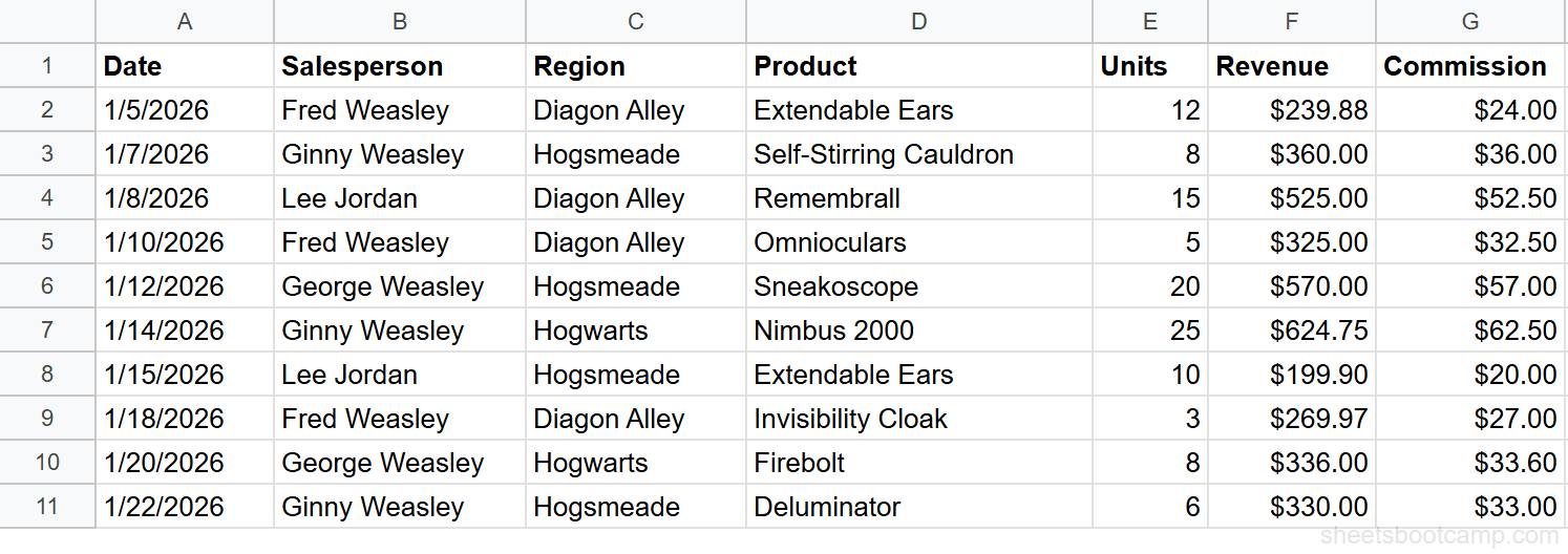
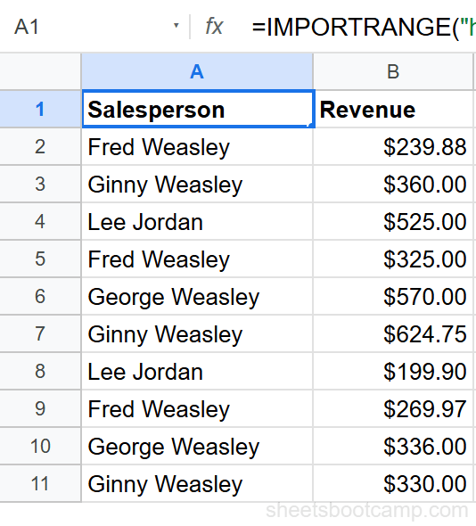
We’ll import sales data from a “Sales Tracking” spreadsheet into a “Monthly Report” spreadsheet. The source contains 10 rows of sales records with Date, Salesperson, Region, Product, Units, Revenue, and Commission.
Sample Data
The source spreadsheet has a sales records table:
Copy the source spreadsheet URL
Open the source spreadsheet (“Sales Tracking”) in your browser. Copy the full URL from the address bar. You need this URL for the IMPORTRANGE formula in the destination spreadsheet.
Enter the IMPORTRANGE formula
Switch to the destination spreadsheet (“Monthly Report”). Select an empty cell and enter the formula:
=IMPORTRANGE("https://docs.google.com/spreadsheets/d/abc123/edit", "Sales Data!A1:G11")Replace abc123 with the actual spreadsheet ID from the URL you copied. Replace Sales Data with the exact tab name in the source file. The range A1:G11 covers the header row plus 10 data rows.
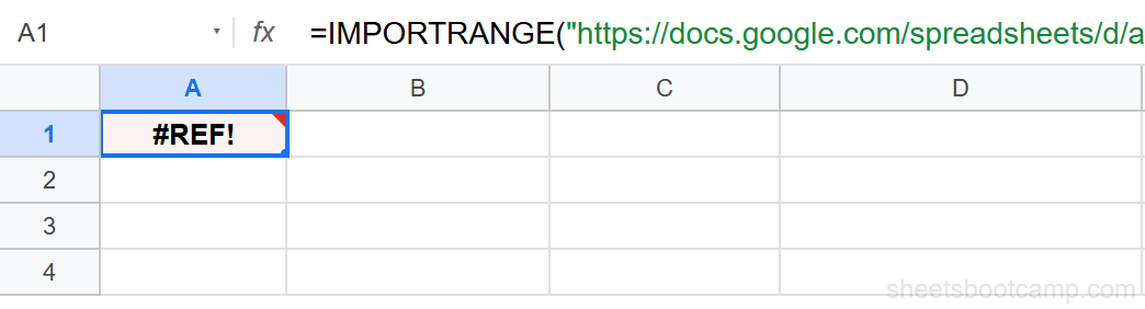
Grant access to the source spreadsheet
The first time you connect two spreadsheets, the cell shows a #REF! error with a tooltip. Hover over the cell and click Allow access in the popup. This grants the destination spreadsheet permission to read data from the source.
You only need to grant access once per source-destination pair. After clicking “Allow access,” the permission persists until someone revokes it. Other users who open the destination spreadsheet don’t need to grant access again.
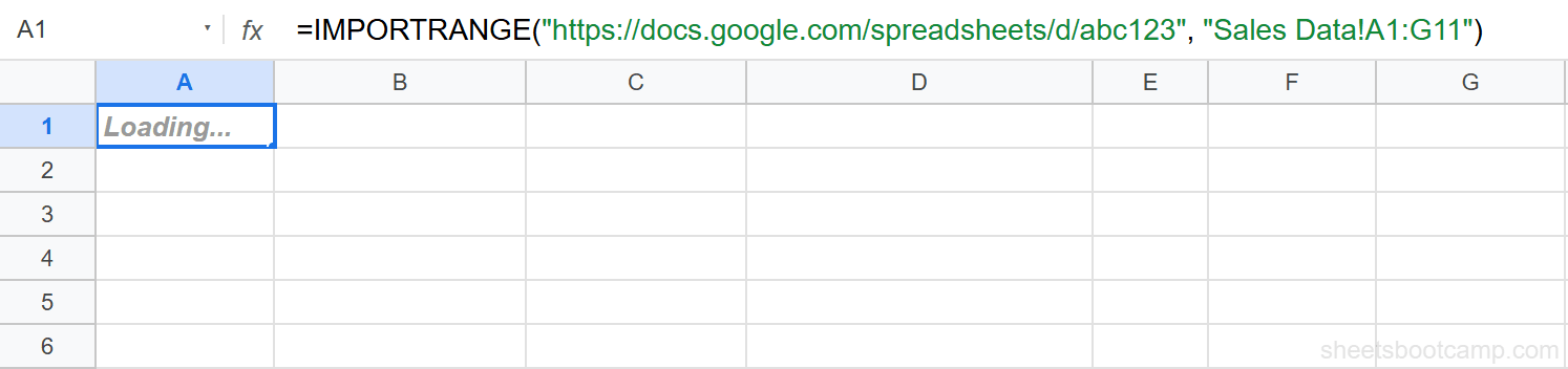
Wait for the data to load
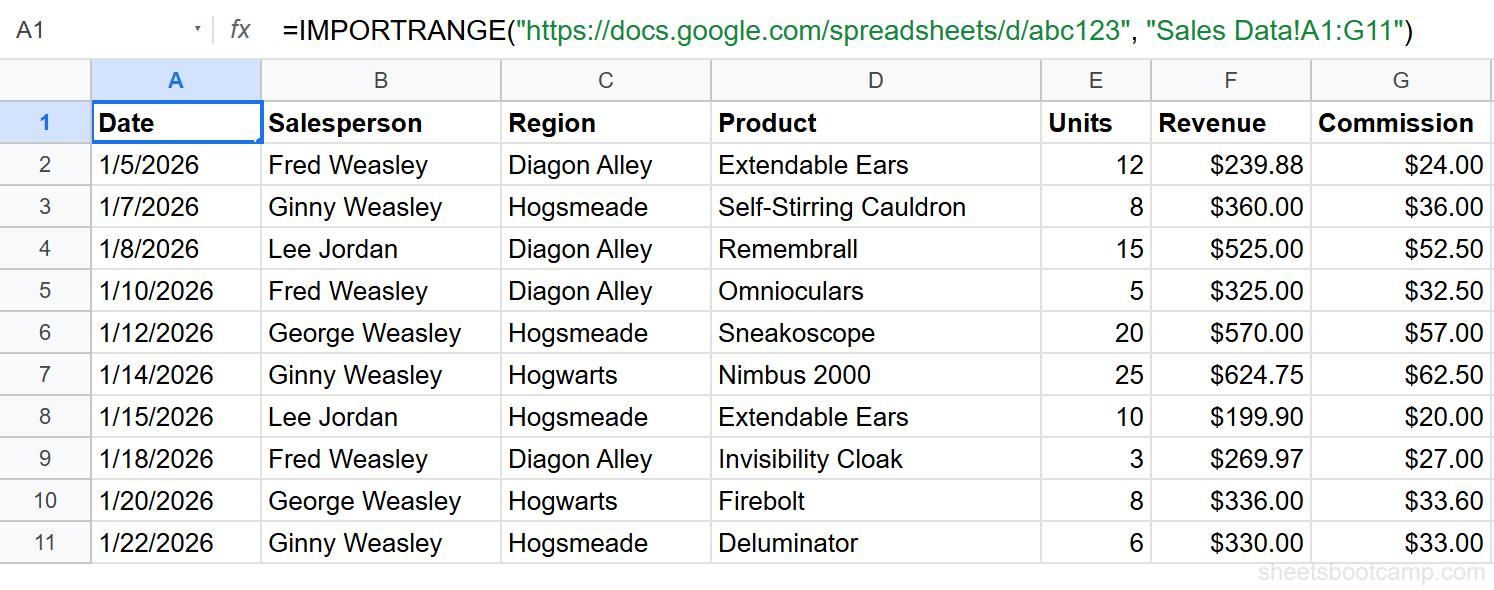
After granting access, the cell briefly shows “Loading…” and then the imported data appears. All 10 rows from the source table populate in the destination, along with the header row.
Verify the imported data
Compare a few values between the source and destination. The imported cells are read-only — you cannot edit them directly. If you need to modify imported data, add formulas in adjacent columns that reference the imported cells.
Use the spreadsheet ID instead of the full URL for shorter formulas. The ID is the long string between /d/ and /edit in the URL. The formula works the same way with either format.
Granting Access
IMPORTRANGE has a built-in permission model. The first time a destination spreadsheet tries to import data from a new source, Google Sheets requires manual approval.
How it works:
- You must have at least view access to the source spreadsheet. If you can’t open the source file yourself, IMPORTRANGE can’t pull data from it either.
- The first IMPORTRANGE call to a new source triggers a #REF! error with an “Allow access” button. Click it once.
- After granting access, the permission applies to all IMPORTRANGE formulas between that source-destination pair. You don’t need to click it again for additional imports from the same source.
- The permission persists until someone removes the connection. Deleting the IMPORTRANGE formula does not revoke access.
If you’re building a shared report, grant access before sharing the destination spreadsheet with other users. That way they see the imported data immediately without encountering the #REF! prompt. For a deeper walkthrough, see the IMPORTRANGE Access Permission guide.
Combining IMPORTRANGE with Other Functions
IMPORTRANGE returns a raw table of data. Wrapping it in other functions lets you filter, sort, or look up specific values from the imported data — all in one formula.
IMPORTRANGE + QUERY
The QUERY function filters and aggregates data using a SQL-like syntax. When you wrap IMPORTRANGE in QUERY, you can filter the imported data before it hits your sheet.
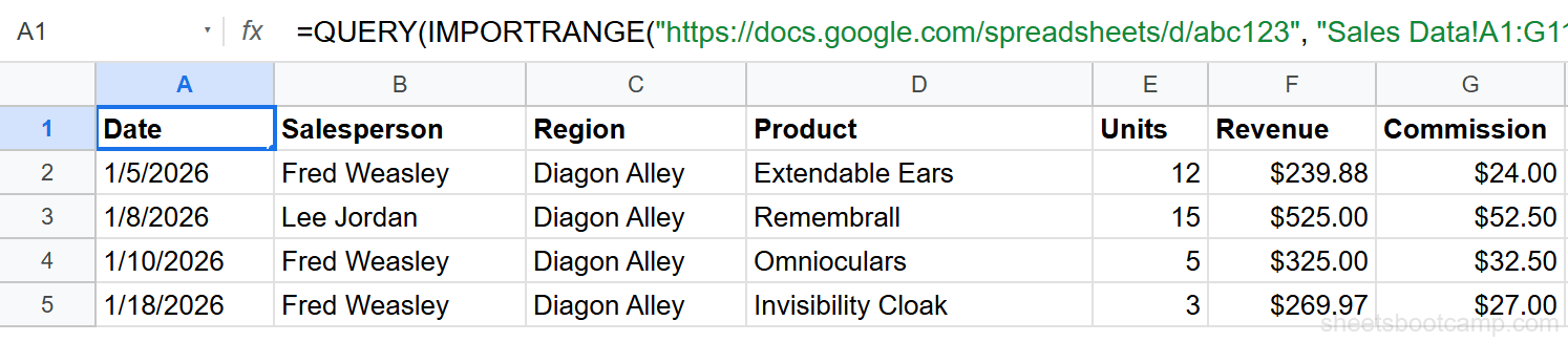
=QUERY(IMPORTRANGE("https://docs.google.com/spreadsheets/d/abc123/edit", "Sales Data!A1:G11"), "SELECT * WHERE Col3 = 'Diagon Alley'")This imports the full sales table, then filters for rows where the Region (column 3) is “Diagon Alley.” The result shows 4 rows: Fred Weasley’s Extendable Ears ($239.88), Lee Jordan’s Remembrall ($525.00), Fred Weasley’s Omnioculars ($325.00), and Fred Weasley’s Invisibility Cloak ($269.97).
When QUERY operates on IMPORTRANGE data, use Col1, Col2, Col3 (numbered column references) instead of column letters like A, B, C. This is because IMPORTRANGE returns a virtual array, not a sheet range with column letters.
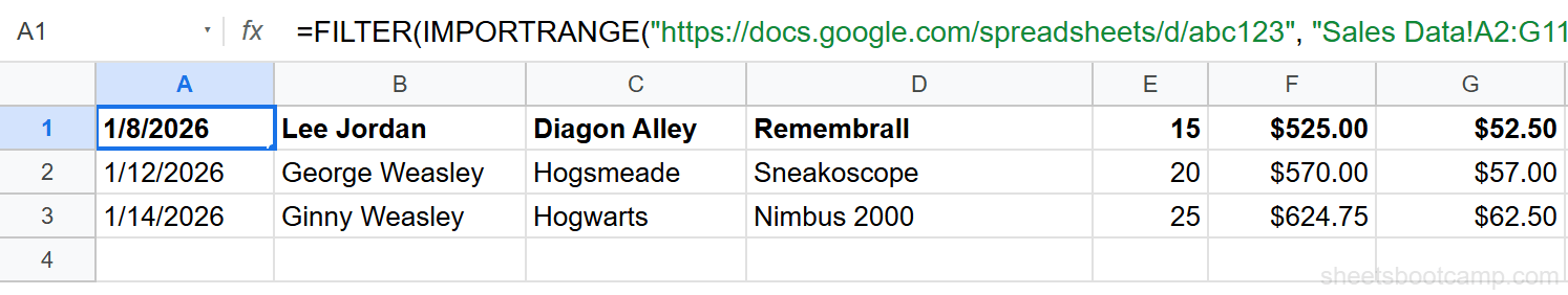
IMPORTRANGE + FILTER
FILTER returns rows from a dataset that match a condition. Wrapping IMPORTRANGE in FILTER imports only the rows you need.
=FILTER(IMPORTRANGE("https://docs.google.com/spreadsheets/d/abc123/edit", "Sales Data!A1:G11"), IMPORTRANGE("https://docs.google.com/spreadsheets/d/abc123/edit", "Sales Data!F2:F11")>400)This imports only rows where Revenue exceeds $400. The result shows 3 rows: Lee Jordan’s Remembrall ($525.00), George Weasley’s Sneakoscope ($570.00), and Ginny Weasley’s Nimbus 2000 ($624.75).
FILTER requires a separate IMPORTRANGE call for the condition column because it needs to evaluate each row individually. If you find this cumbersome, use QUERY instead — it handles filtering with a single import.
IMPORTRANGE + VLOOKUP
You can use IMPORTRANGE as the range argument in VLOOKUP to look up a value in an external spreadsheet:
=VLOOKUP("Remembrall", IMPORTRANGE("https://docs.google.com/spreadsheets/d/abc123/edit", "Sales Data!D2:F11"), 3, FALSE)This searches the Product column in the external spreadsheet for “Remembrall” and returns $525.00. For more patterns, see the IMPORTRANGE with VLOOKUP guide.
Practical Examples
Example 1: Import a Full Table
The step-by-step tutorial above covers this case. You import the entire A1:G11 range, which brings in the header row and all 10 data rows. This is the most common IMPORTRANGE use case.
Example 2: Import Specific Columns
You only need the Salesperson (column B) and Revenue (column F) from the source. Use QUERY to select specific columns from the imported data:
=QUERY(IMPORTRANGE("https://docs.google.com/spreadsheets/d/abc123/edit", "Sales Data!A1:G11"), "SELECT Col2, Col6")This returns a two-column table with Salesperson and Revenue for all 10 rows, without the other five columns.
Example 3: Import from a Named Range
If the source spreadsheet uses named ranges, you can reference them directly in the range_string:
=IMPORTRANGE("https://docs.google.com/spreadsheets/d/abc123/edit", "SalesTotal")Replace SalesTotal with the actual named range in the source file. This is cleaner than specifying "Sales Data!F12" because the named range stays valid even if the source table moves.
Common Errors and Fixes
#REF! Error: Access Not Granted
This is the most common IMPORTRANGE error. It means the destination spreadsheet doesn’t have permission to read from the source.
Fix: Hover over the cell showing the error. Click Allow access in the popup tooltip. If the popup doesn’t appear, delete the formula, re-enter it, and press Enter again.
#REF! Error: Invalid Range String
The range_string doesn’t match anything in the source spreadsheet. Common causes:
- The sheet tab name is misspelled. “Sales Data” is different from “sales data” — tab names are case-sensitive.
- The tab has been renamed or deleted in the source file.
- The cell range exceeds the source sheet’s dimensions.
Fix: Open the source spreadsheet and copy the exact tab name. Double-check the cell range against the actual data.
#VALUE! Error: Bad URL
The spreadsheet URL is wrong, malformed, or points to a file that doesn’t exist.
Fix: Open the source spreadsheet in your browser and copy the URL directly from the address bar. Verify the URL opens the correct file before pasting it into the formula.
”Loading…” That Never Resolves
The cell shows “Loading…” indefinitely. This happens with large datasets, slow connections, or when Google’s servers are under heavy load.
Fix: Wait a few minutes. If it persists, try reducing the import range (import fewer columns or rows). Check your internet connection. As a last resort, delete the formula and re-enter it.
For more on refresh behavior, see the IMPORTRANGE Auto-Update guide.
Imported Data Doesn’t Update
IMPORTRANGE refreshes automatically, but not instantly. Changes in the source can take a few seconds to a few minutes to appear in the destination. Large spreadsheets with many IMPORTRANGE formulas take longer.
If the data seems stale, try refreshing the page or making a small edit in the destination spreadsheet to trigger a recalculation.
Performance Tips
IMPORTRANGE recalculates whenever the source spreadsheet changes or the destination sheet refreshes. A few practices keep it fast:
-
Limit the range. Import
A1:G11instead ofA:G. Full-column references force Sheets to scan every row, even empty ones. -
Avoid chaining IMPORTRANGE calls. Spreadsheet A imports from B, and B imports from C. Each link adds latency and increases the chance of errors. Import directly from the source whenever possible.
-
Reduce the number of IMPORTRANGE formulas. One formula that imports a 500-row table is faster than 500 formulas that each import one row. Consolidate imports into larger ranges and use helper formulas to extract what you need.
-
Large imports (10,000+ rows) are slow by design. If you need that much data, consider using Google Apps Script or a connected sheet in BigQuery instead.
For more optimization strategies, see the IMPORTRANGE Performance guide.
Tips and Best Practices
-
Use the spreadsheet ID instead of the full URL. The ID is shorter, cleaner, and less likely to break if Google changes the URL format. Find it between
/d/and/editin the spreadsheet URL. -
Grant access proactively before sharing. If you’re building a report for others, open the destination file yourself and click “Allow access” first. Your colleagues won’t have to deal with the #REF! prompt.
-
Import only the columns you need. Wrap IMPORTRANGE in QUERY with a SELECT clause to pull specific columns. This keeps your destination sheet cleaner and reduces the data transferred.
-
Wrap in IFERROR for graceful fallbacks. If the source is temporarily unavailable, IFERROR prevents an ugly error message:
=IFERROR(IMPORTRANGE("url", "Sales Data!A1:G11"), "Data temporarily unavailable")-
Document source spreadsheet URLs in a notes cell. Keep a cell or a hidden sheet that lists every source URL and what data it provides. When something breaks six months later, you’ll know where to look.
-
Combine with QUERY for server-side filtering. Instead of importing everything and filtering in the destination, let QUERY handle the filtering inside the IMPORTRANGE call. This reduces the amount of data transferred between spreadsheets.
Related Google Sheets Tutorials
- IMPORTRANGE Access Permission — How the permission model works and troubleshooting access issues
- IMPORTRANGE with VLOOKUP — Look up values from an external spreadsheet without copying data
- IMPORTRANGE Auto-Update — How refresh timing works and forcing updates
- IMPORTRANGE from Multiple Tabs — Import data from several tabs in the same source file
- VLOOKUP Complete Guide — Look up values in a table by searching the first column
- QUERY Function Guide — Filter, sort, and aggregate data using SQL-like syntax
- IF Function Guide — Conditional logic for evaluating true/false conditions per row
Frequently Asked Questions
How do I use IMPORTRANGE in Google Sheets?
Enter =IMPORTRANGE("spreadsheet_url", "SheetName!A1:G11") in an empty cell. The first argument is the source spreadsheet URL or ID, and the second is the sheet name and range in quotes. Grant access when prompted, and the data appears in your sheet.
Why does IMPORTRANGE show #REF?
The #REF! error usually means you have not granted access to the source spreadsheet. Hover over the error cell and click “Allow access” in the popup. If the error persists, check that the range string and sheet name are correct.
Does IMPORTRANGE update automatically?
Yes. IMPORTRANGE creates a live link between two spreadsheets. When the source data changes, the destination updates automatically. There can be a short delay depending on the size of the imported range.
Can I use IMPORTRANGE with VLOOKUP?
Yes. Use IMPORTRANGE as the range argument in VLOOKUP: =VLOOKUP(A2, IMPORTRANGE("url", "Sheet1!A1:C100"), 2, FALSE). This looks up a value in an external spreadsheet without copying the data manually.
How do I import data from multiple tabs?
Use a separate IMPORTRANGE formula for each tab. Each formula references the same spreadsheet URL but a different sheet name in the range string. For example, one formula imports "Sales!A1:G10" and another imports "Inventory!A1:D20".
Is there a limit to how much data IMPORTRANGE can pull?
Google Sheets has a cell limit of 10 million cells per spreadsheet. IMPORTRANGE counts toward this limit in the destination sheet. Large imports (10,000+ rows) work but can be slow. Import only the columns and rows you need.
Can I use IMPORTRANGE with a private spreadsheet?
You must have at least view access to the source spreadsheet. If the source is private and you do not have access, IMPORTRANGE returns a #REF! error. Ask the spreadsheet owner to share it with your Google account.
How do I remove the Allow access prompt?
You cannot skip the prompt entirely. It appears the first time a destination spreadsheet connects to a new source. Click “Allow access” once, and the permission persists for that source-destination pair until revoked.