Does IMPORTRANGE Auto-Update? Sync Explained
Learn how IMPORTRANGE auto-update works in Google Sheets, how to force a refresh, and what to do when imported data stops syncing between spreadsheets.
Sheets Bootcamp
May 27, 2026
IMPORTRANGE in Google Sheets creates a live connection between two spreadsheets, and it does auto-update. When the source data changes, the destination refreshes automatically without any manual intervention. Understanding how that refresh cycle works, and what can interrupt it, saves you from staring at stale numbers wondering what went wrong.
This guide covers how IMPORTRANGE auto-update works in Google Sheets, how to force a refresh when you need it, and how to troubleshoot when syncing stops.
In This Guide
- How IMPORTRANGE Auto-Update Works
- Step-by-Step: Verify IMPORTRANGE Is Updating
- How to Force IMPORTRANGE to Refresh
- When IMPORTRANGE Stops Updating
- Tips and Best Practices
- Related Google Sheets Tutorials
- Frequently Asked Questions
How IMPORTRANGE Auto-Update Works
IMPORTRANGE does not copy data. It maintains a live link to the source spreadsheet and fetches the latest values whenever Google Sheets triggers a recalculation.
When someone edits the source spreadsheet, Google Sheets queues a refresh on any destination file that references it via IMPORTRANGE. That refresh typically takes one to five minutes. You do not need to do anything to trigger it. The sync happens in the background.
Here is the standard formula:
=IMPORTRANGE("spreadsheet_url", "Sheet1!A1:D10")The first argument is the source spreadsheet URL or ID. The second is the range string including the sheet name. Once you grant access permissions, the link is persistent and updates without intervention.
IMPORTRANGE is not a real-time push. It syncs on recalculation, not on keystroke. Expect a delay of up to a few minutes after a source change before the destination reflects it.
Step-by-Step: Verify IMPORTRANGE Is Updating
Use this process to confirm your IMPORTRANGE formula is actively syncing between spreadsheets.
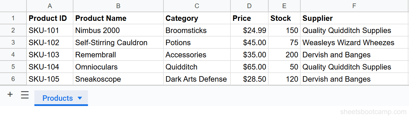
Open both spreadsheets
Open the source spreadsheet in one browser tab and the destination spreadsheet in another. The source contains a product inventory with data in columns A through F. The destination has an IMPORTRANGE formula pulling that data.
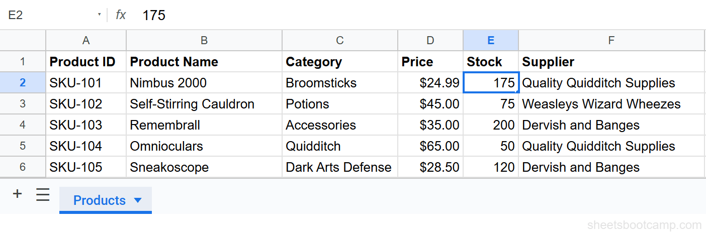
Make a change in the source
In the source spreadsheet, change the Stock value for SKU-101 (Nimbus 2000) from 150 to 175. Google Sheets saves the change automatically.
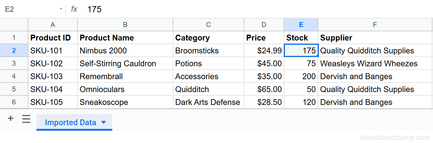
Switch to the destination and verify
Wait 30 to 60 seconds, then switch to the destination spreadsheet. Check the cell that corresponds to SKU-101’s Stock value. If IMPORTRANGE is working, it now displays 175 instead of 150.
Force a refresh if the value has not changed
If the destination still shows 150 after a couple of minutes, press Ctrl+Shift+F9 on Windows or Cmd+Shift+F9 on Mac. This forces Google Sheets to recalculate all formulas in the file, including IMPORTRANGE. The cell should update within seconds.
You can also force a single-cell refresh by clicking the IMPORTRANGE cell, pressing F2, and pressing Enter. This re-evaluates that one formula.
How to Force IMPORTRANGE to Refresh
Keyboard Shortcut
Ctrl+Shift+F9 (Windows) or Cmd+Shift+F9 (Mac) forces an immediate recalculation of the entire spreadsheet. This is the fastest way to pull the latest data from a source file.
Re-Enter the Formula
Click the cell containing IMPORTRANGE, press F2 to enter edit mode, and press Enter. This re-evaluates the formula without changing it.
Volatile Function Workaround
Some users wrap IMPORTRANGE with NOW() to encourage more frequent refreshes:
=IF(NOW()>0, IMPORTRANGE("spreadsheet_url", "Sheet1!A1:D10"), "")NOW() is a volatile function that recalculates whenever the spreadsheet recalculates. The IF condition always evaluates to TRUE (NOW() always returns a positive number), so the IMPORTRANGE result always displays. This is a workaround, not an officially supported mechanism, and it increases calculation load on the file.
For most use cases, the automatic sync is sufficient. Use the volatile function trick only when your data needs to stay current within minutes and manual refreshes are not practical.
Spreadsheet Calculation Settings
Google Sheets has a calculation setting under File > Settings > Calculation. The default Recalculation value is “On change.” This setting controls volatile functions like NOW() and TODAY() but does not directly control IMPORTRANGE’s sync mechanism. IMPORTRANGE has its own refresh cycle managed by Google’s servers.
When IMPORTRANGE Stops Updating
If your IMPORTRANGE data appears frozen, one of these causes is usually responsible.
Access Permissions Revoked
When the source spreadsheet owner changes sharing settings, IMPORTRANGE loses access. The formula displays a #REF! error with “You don’t have permission.” The owner needs to restore access, and you may need to click Allow access again.
Source Spreadsheet Moved or Deleted
If the source file was deleted, moved to Trash, or its URL changed, IMPORTRANGE cannot find it. Update the spreadsheet URL in your formula to point to the new location.
Too Many IMPORTRANGE Calls
Google Sheets handles IMPORTRANGE connections through a shared quota. Loading dozens of IMPORTRANGE formulas in one file increases the chance of delays or failures. Consolidate ranges where possible. One IMPORTRANGE pulling A1:Z1000 is more efficient than ten formulas pulling separate columns.
Dataset Exceeds Cell Limits
Google Sheets has a limit of 10 million cells per spreadsheet. IMPORTRANGE output counts toward this limit in the destination. If either file is near the limit, IMPORTRANGE may fail or stall. Check file size under Tools > Spreadsheet statistics.
Incorrect Range String
A typo in the sheet name or range reference causes IMPORTRANGE to error immediately. Sheet names in the range string must match the source tab name exactly, including capitalization. “Q1 Sales” and “q1 sales” are different tabs.
If your IMPORTRANGE formula shows a spinning loading indicator for more than five minutes, the source spreadsheet may be too large or the connection quota may be exhausted. Try reducing the range you are importing to only the columns and rows you need.
Tips and Best Practices
-
Import only the columns you need. Pulling
A:Zwhen you need columns A and C wastes cell quota and increases load time. Use IMPORTRANGE with FILTER or QUERY to narrow the import at the source level. -
Centralize imports in a staging sheet. Pull all IMPORTRANGE data into a single hidden sheet named
_import. Build your working views using formulas that reference that local sheet. This reduces the number of live external connections and makes the spreadsheet faster. -
Use the spreadsheet ID instead of the full URL. The ID is the string between
/d/and/editin the URL. It looks like a long random string. A shorter formula is easier to read and less prone to pasting errors. -
Check connection status by hovering. Hover over an IMPORTRANGE cell to see a tooltip. “Loading…” means the formula is actively fetching. A #REF! error with a message tells you what went wrong.
-
Avoid nesting IMPORTRANGE inside complex array formulas on large ranges. Combining IMPORTRANGE with ARRAYFORMULA or wrapping it inside VLOOKUP multiplies the calculation cost. Use a helper range pattern: import the data first, then run lookups against the local copy. The VLOOKUP with IMPORTRANGE article covers this approach.
Related Google Sheets Tutorials
- IMPORTRANGE in Google Sheets: Complete Guide - Full reference for syntax, use cases, and troubleshooting
- Fix IMPORTRANGE Access Permission - Resolve #REF! errors caused by permission issues
- VLOOKUP with IMPORTRANGE - Look up values across spreadsheets using both functions together
- IMPORTRANGE from Multiple Tabs - Import data from several tabs in one source spreadsheet
- IFERROR Function - Wrap IMPORTRANGE errors so your sheet stays clean
Frequently Asked Questions
Does IMPORTRANGE update automatically in Google Sheets?
Yes. IMPORTRANGE creates a live link between spreadsheets and refreshes automatically whenever the source data changes. Updates typically appear within a few minutes, though large datasets may take longer.
How often does IMPORTRANGE refresh?
IMPORTRANGE refreshes whenever the source spreadsheet changes or whenever Google Sheets recalculates the destination file. There is no fixed interval. Changes propagate as they happen, usually within one to five minutes.
How do I force IMPORTRANGE to update?
Press Ctrl+Shift+F9 on Windows or Cmd+Shift+F9 on Mac to force recalculation of all formulas in the destination spreadsheet, including IMPORTRANGE. You can also click the IMPORTRANGE cell, press F2, and press Enter.
Why is my IMPORTRANGE not updating?
Common causes include the source spreadsheet being deleted or moved, access permissions being revoked, too many IMPORTRANGE calls in one file, or the dataset exceeding the 10 million cell limit. Check the formula for a #REF! or loading error first.
Does IMPORTRANGE work in real time?
Not exactly. IMPORTRANGE does not push updates the instant a cell changes. It syncs when Google Sheets triggers a recalculation, typically within a few minutes of a change in the source file.