IMPORTRANGE with FILTER in Google Sheets

IMPORTRANGE pulls data from another Google Sheets spreadsheet. Wrapping it in FILTER lets you import only the rows that match a condition, so you are not hauling in a thousand rows when you need twenty. When your source data is large and you want targeted results in the destination, IMPORTRANGE with FILTER is the formula pattern to reach for.

We will cover how the combination works, walk through a step-by-step example, and show three practical variations including multiple conditions and sorting.

In This Guide

• How FILTER and IMPORTRANGE Work Together
• Step-by-Step: Filter Imported Data
• Practical Examples
• FILTER vs QUERY with IMPORTRANGE
• Common Errors
• Tips and Best Practices
• Related Google Sheets Tutorials
• Frequently Asked Questions

How FILTER and IMPORTRANGE Work Together

FILTER takes two arguments: an array to return, and a condition that determines which rows to include. When you use IMPORTRANGE as the array, FILTER evaluates the imported data directly without you needing to store it anywhere first.

The structure looks like this:

=FILTER(IMPORTRANGE("url", "range"), condition)

The condition must be an array the same height as the imported range. The most reliable approach is to use a second IMPORTRANGE that pulls only the column you want to filter on.

For example, to filter a product table where the Stock column is column E:

=FILTER(IMPORTRANGE("url", "Sheet1!A2:F101"), IMPORTRANGE("url", "Sheet1!E2:E101") > 100)

The first IMPORTRANGE returns all six columns. The second returns only column E. FILTER compares each E value against 100 and keeps the rows where the result is TRUE.

Step-by-Step: Filter Imported Data

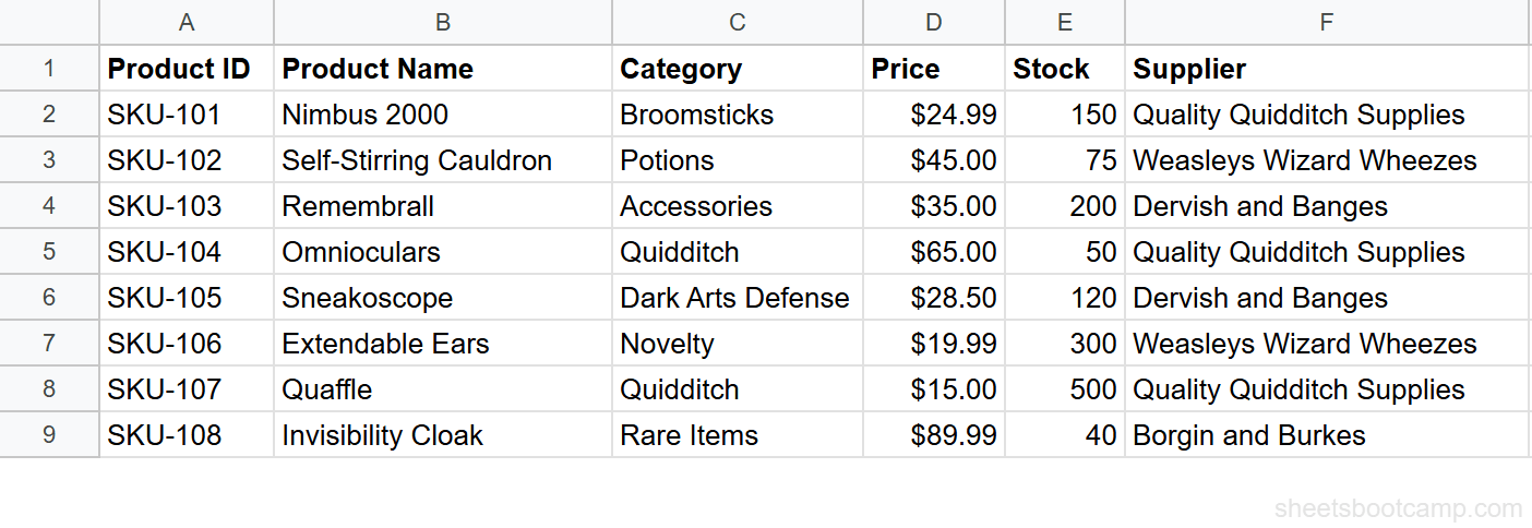
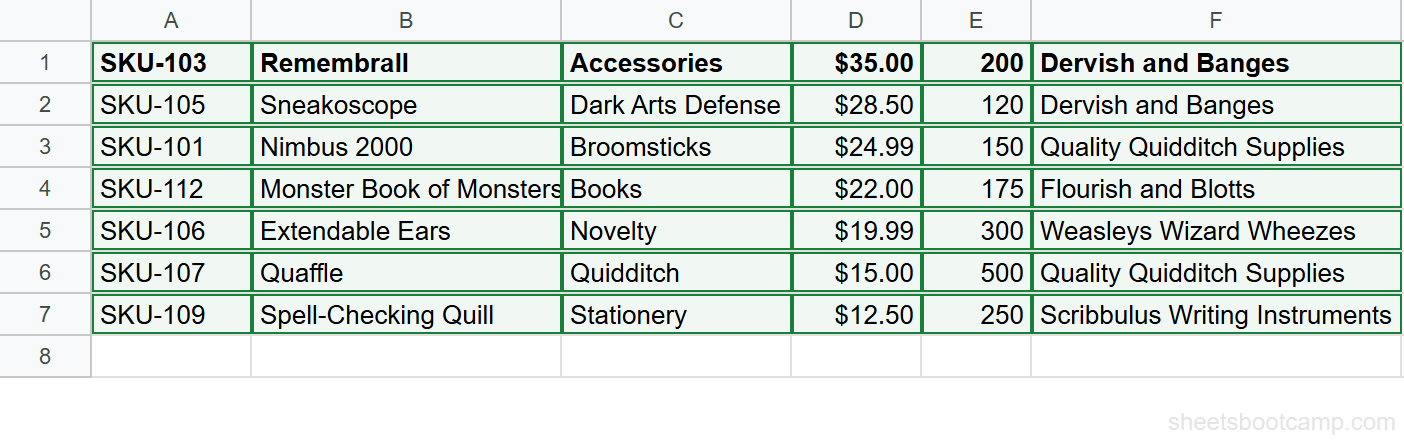
We will work with a product inventory spreadsheet. The source has 12 rows of products with columns Product ID, Product Name, Category, Price, Stock, and Supplier. The goal: import only products with Stock greater than 100.

Sample Source Data

The source spreadsheet contains the product inventory with Stock values ranging from 40 to 500:

In the destination spreadsheet, select cell A1 and enter the base IMPORTRANGE. This confirms the connection is working before you add FILTER on top of it.

=IMPORTRANGE("https://docs.google.com/spreadsheets/d/abc123/edit", "Sheet1!A1:F13")

Replace abc123 with the actual spreadsheet ID from the source URL. If the cell shows a #REF! error, hover over it and click Allow access. Once the data loads, delete this formula and move to the next step.

Stock is in column E of the source data, rows 2 through 13 (excluding the header). The condition range you will use is Sheet1!E2:E13.

If you plan to add more rows to the source later, extend the range: Sheet1!E2:E1000. FILTER ignores blank rows at the bottom automatically.

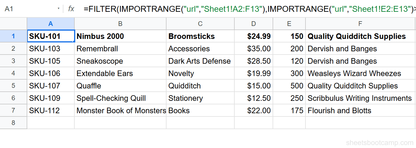
Select cell A1 in the destination and enter the full formula:

=FILTER(IMPORTRANGE("https://docs.google.com/spreadsheets/d/abc123/edit", "Sheet1!A2:F13"), IMPORTRANGE("https://docs.google.com/spreadsheets/d/abc123/edit", "Sheet1!E2:E13") > 100)

The first IMPORTRANGE is the array FILTER returns. The second IMPORTRANGE is the condition. FILTER checks each value in column E and keeps the row if it is greater than 100.

The formula returns 7 rows. Products with Stock of 75 or fewer (Self-Stirring Cauldron at 75, Omnioculars at 50, Invisibility Cloak at 40, and Deluminator at 60) are excluded. Nimbus 2000 (150), Remembrall (200), Sneakoscope (120), Extendable Ears (300), Quaffle (500), Spell-Checking Quill (250), and Monster Book of Monsters (175) appear in the results.

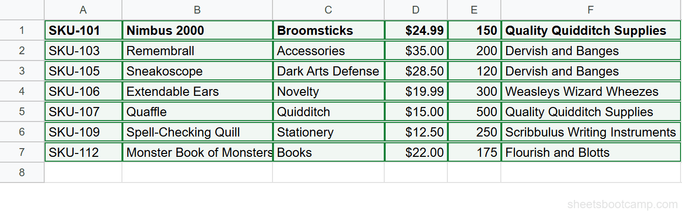
The header row is not included because we started the imported range at row 2. Add a manual header row above the formula cell if you want labels.

Practical Examples

Example 1: Filter by Text Value

The product inventory has a Category column in column C. To import only rows where Category is “Broomsticks”:

=FILTER(IMPORTRANGE("https://docs.google.com/spreadsheets/d/abc123/edit", "Sheet1!A2:F13"), IMPORTRANGE("https://docs.google.com/spreadsheets/d/abc123/edit", "Sheet1!C2:C13") = "Broomsticks")

This returns two rows: Nimbus 2000 ($24.99, Stock 150) and Firebolt ($42.00, Stock 85). Text comparisons in FILTER are case-insensitive, so “broomsticks” and “BROOMSTICKS” return the same results.

To expand to multiple categories, use the OR pattern:

=FILTER(IMPORTRANGE("https://docs.google.com/spreadsheets/d/abc123/edit", "Sheet1!A2:F13"), (IMPORTRANGE("https://docs.google.com/spreadsheets/d/abc123/edit", "Sheet1!C2:C13") = "Broomsticks") + (IMPORTRANGE("https://docs.google.com/spreadsheets/d/abc123/edit", "Sheet1!C2:C13") = "Quidditch"))

The + operator acts as OR: rows where Category is “Broomsticks” OR “Quidditch” are returned. This gives you Nimbus 2000, Omnioculars, Quaffle, and Firebolt.

Example 2: Filter by Multiple Conditions (AND)

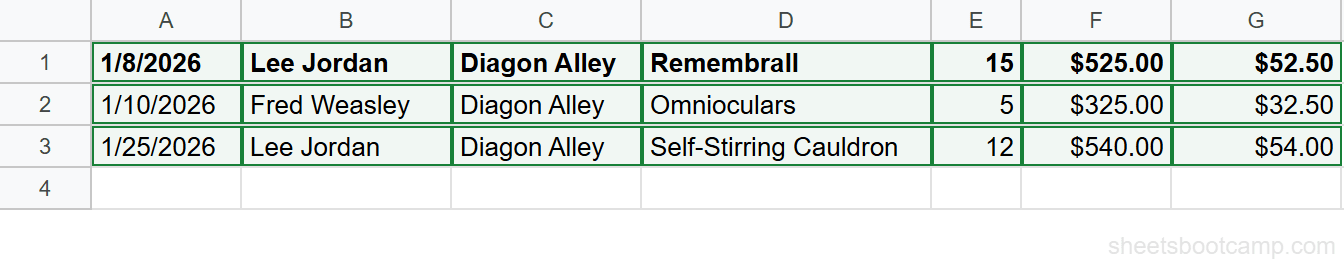
Using the sales records spreadsheet, you want only rows where Region is “Diagon Alley” AND Revenue is greater than $300. Region is column C, Revenue is column F.

=FILTER(IMPORTRANGE("https://docs.google.com/spreadsheets/d/abc123/edit", "Sales!A2:G19"), (IMPORTRANGE("https://docs.google.com/spreadsheets/d/abc123/edit", "Sales!C2:C19") = "Diagon Alley") * (IMPORTRANGE("https://docs.google.com/spreadsheets/d/abc123/edit", "Sales!F2:F19") > 300))

The * operator acts as AND: both conditions must be TRUE for a row to appear. From the sales records, this returns:

• Lee Jordan, 1/8/2026, Remembrall, $525.00
• Fred Weasley, 1/10/2026, Omnioculars, $325.00
• Fred Weasley, 1/18/2026, Invisibility Cloak, $269.97 — wait, $269.97 is below $300, so this row is excluded.
• Lee Jordan, 1/25/2026, Self-Stirring Cauldron, $540.00
• Ginny Weasley, 1/30/2026, Monster Book of Monsters, $220.00 — also excluded, below $300.

The formula returns Lee Jordan ($525.00 on 1/8), Fred Weasley ($325.00 on 1/10), and Lee Jordan ($540.00 on 1/25).

Example 3: Combine FILTER with SORT

To filter and sort the results in one formula, wrap the entire FILTER expression inside SORT. This example returns products with Stock greater than 100, sorted by Price from highest to lowest (column 4 of the returned array, descending):

=SORT(FILTER(IMPORTRANGE("https://docs.google.com/spreadsheets/d/abc123/edit", "Sheet1!A2:F13"), IMPORTRANGE("https://docs.google.com/spreadsheets/d/abc123/edit", "Sheet1!E2:E13") > 100), 4, FALSE)

SORT takes the FILTER output as its array. The second argument (4) references the 4th column of the returned result, which is Price. FALSE means descending order. The 7 qualifying products sorted by Price from highest to lowest: Remembrall ($35.00), Sneakoscope ($28.50), Nimbus 2000 ($24.99), Monster Book of Monsters ($22.00), Extendable Ears ($19.99), Quaffle ($15.00), Spell-Checking Quill ($12.50).

FILTER vs QUERY with IMPORTRANGE

Both FILTER and QUERY work with IMPORTRANGE. They solve the same problem from different angles.

FILTER uses native Google Sheets array logic. Conditions use standard operators (=, >, <, *, +). The syntax is predictable if you already know Google Sheets formulas. FILTER returns rows only. It cannot group, count, or aggregate.

QUERY accepts a SQL-like string as its second argument. It can filter, sort, group, and aggregate in one formula. For simple row filtering, QUERY requires more syntax. For summary tables or computed columns, QUERY handles things FILTER cannot.

For the same “Stock > 100” filter, QUERY looks like this:

=QUERY(IMPORTRANGE("https://docs.google.com/spreadsheets/d/abc123/edit", "Sheet1!A1:F13"), "SELECT * WHERE Col5 > 100")

QUERY uses Col5 to reference the 5th column of the imported range. FILTER uses a second IMPORTRANGE for the same column. Neither is strictly better. Use FILTER when you know Google Sheets array formulas. Use QUERY when you need aggregation or know SQL syntax. See the QUERY with IMPORTRANGE article for full examples.

Common Errors

#N/A — No Matching Rows

FILTER returns #N/A when the condition matches zero rows. The formula is correct, but your filter is too strict or the source data changed.

Fix: Wrap the formula in IFERROR to return a readable message:

=IFERROR(FILTER(IMPORTRANGE("url", "range"), IMPORTRANGE("url", "cond-range") > 100), "No products match this filter")

#REF! — Access Not Granted

If you see #REF! immediately after entering the formula, the destination spreadsheet does not have permission to read from the source. Hover over the error cell and click Allow access. See IMPORTRANGE access permissions for details.

Condition Array Size Mismatch

FILTER requires the condition array to have exactly the same number of rows as the main array. If your main range is A2:F13 (12 rows) but your condition range is E2:E10 (9 rows), the formula breaks.

Fix: Make both ranges the same size. If you are extending ranges to accommodate future rows, extend both to the same endpoint: A2:F1000 and E2:E1000.

Column Count Changes in the Source

If someone adds or removes a column in the source spreadsheet, the column references inside FILTER shift. A condition on column E may now point to column F.

Fix: Use named ranges in the source spreadsheet and reference the name in IMPORTRANGE instead of a hard-coded column letter.

Tips and Best Practices

1. Extend your ranges beyond current data. Use A2:F1000 instead of A2:F13. New rows added to the source automatically appear in the filtered output without updating the formula.

2. Shorten the URL to the spreadsheet ID. Extract the ID between /d/ and /edit. A formula with a 44-character ID is easier to read and edit than one with a 200-character URL.

3. Store repeated URLs in a cell. If you use the same source URL across multiple formulas, enter the URL once in a cell (for example, cell Z1) and reference it: =FILTER(IMPORTRANGE(Z1, "Sheet1!A2:F1000"), IMPORTRANGE(Z1, "Sheet1!E2:E1000") > 100). Update the URL in one place when the source changes.

4. Add headers manually above the formula. FILTER returns data rows only. Put your column labels in the row above the formula cell. This avoids including the header row in the imported range and prevents the header from appearing inside filter results.

5. Combine with IMPORTRANGE auto-update behavior. IMPORTRANGE refreshes on a schedule, not instantly. If your filtered output needs to reflect real-time changes, check the source spreadsheet’s recalculation settings and the IMPORTRANGE refresh interval.

Related Google Sheets Tutorials

• IMPORTRANGE: The Complete Guide — Full syntax, parameters, and examples for pulling data between spreadsheets
• IMPORTRANGE Access Permission — Fix the #REF! error and manage connection grants between spreadsheets
• VLOOKUP with IMPORTRANGE — Look up specific values from an external spreadsheet using VLOOKUP
• QUERY with IMPORTRANGE — Filter and aggregate imported data using SQL-like QUERY syntax
• IMPORTRANGE Auto-Update — Understand how and when IMPORTRANGE refreshes data from the source

Frequently Asked Questions

Can you use FILTER with IMPORTRANGE in Google Sheets?

Yes. Wrap IMPORTRANGE inside FILTER: =FILTER(IMPORTRANGE(url, range), condition). The condition references columns from the imported data by index using OFFSET or by wrapping another IMPORTRANGE for just the condition column.

Why does FILTER with IMPORTRANGE return #N/A?

The #N/A error means no rows matched your condition. FILTER returns #N/A when the condition array has no TRUE values. Wrap the formula in IFERROR to return a custom message instead: =IFERROR(FILTER(IMPORTRANGE(...), ...), "No results").

How do I filter IMPORTRANGE by multiple conditions?

Use multiplication (*) for AND logic and addition (+) for OR logic inside FILTER. For example: =FILTER(IMPORTRANGE(url, range), (condition1) * (condition2)) requires both conditions to be true.

Is FILTER or QUERY better with IMPORTRANGE?

FILTER handles numeric and text conditions with native Google Sheets syntax. QUERY uses SQL-like syntax and can group and aggregate data. For simple row filtering, FILTER is faster to write. For summaries and sorting, QUERY is more flexible.

Does FILTER update automatically when source data changes?

Yes. IMPORTRANGE pulls live data from the source spreadsheet, and FILTER evaluates the result on each recalculation. When the source changes, the filtered output updates automatically, subject to the normal IMPORTRANGE refresh interval.