IMPORTRANGE from Multiple Tabs in Google Sheets

IMPORTRANGE in Google Sheets pulls data from an external spreadsheet — but one formula can only reference one tab at a time. When you need to import from multiple tabs, you have a few options: separate formulas for each tab, stacked arrays using curly braces, or QUERY to filter and combine the results. This article covers all three approaches using a source spreadsheet with a Sales tab and an Inventory tab.

In This Guide

• How IMPORTRANGE References Tabs
• Step-by-Step: Import from Multiple Tabs
• Stacking Data from Multiple Tabs
• Combining IMPORTRANGE with QUERY
• Common Errors
• Tips and Best Practices
• Related Google Sheets Tutorials
• Frequently Asked Questions

How IMPORTRANGE References Tabs

IMPORTRANGE takes two arguments: a spreadsheet URL and a range string.

=IMPORTRANGE("spreadsheet_url", "range_string")

The range string is where you specify the tab. The format is:

"TabName!CellRange"

For example, to import A1:G10 from a tab named Sales:

=IMPORTRANGE("https://docs.google.com/spreadsheets/d/SOURCE_ID/edit", "Sales!A1:G10")

A few rules for tab names in the range string:

• Exact match required. The tab name is case-sensitive. “sales” and “Sales” are different tabs.
• Spaces work as-is. If your tab is named “Sales Data”, write "Sales Data!A1:G10". The outer quotes around the full range string handle it. You do not need extra escaping.
• No tab name defaults to the first tab. If you write "A1:G10" with no tab name, IMPORTRANGE imports from the first tab in the source spreadsheet.

Step-by-Step: Import from Multiple Tabs

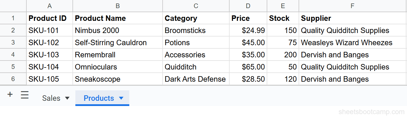
We have a source spreadsheet with two tabs. The Sales tab has transaction records (columns: Date, Product, SKU, Quantity, Unit Price, Total, Region). The Inventory tab has stock levels (columns: SKU, Product, Category, Stock, Reorder Point, Supplier).

In your destination spreadsheet, select an empty cell. Enter:

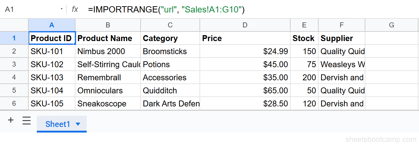
=IMPORTRANGE("https://docs.google.com/spreadsheets/d/SOURCE_ID/edit", "Sales!A1:G10")

The cell shows a #REF! error. This is expected. Hover over the cell and click Allow access. This grants the destination spreadsheet permission to read from the source file. You only do this once per source-destination pair — not once per tab.

After you click Allow access, the Sales data populates starting from that cell.

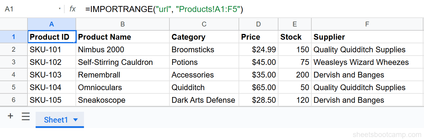
Select a different empty cell — somewhere with enough room that it won’t overlap with the Sales data. Enter:

=IMPORTRANGE("https://docs.google.com/spreadsheets/d/SOURCE_ID/edit", "Inventory!A1:F5")

This time, no Allow access prompt appears. The access was already granted when you clicked it for the Sales import. The Inventory data loads immediately.

Check that the row counts match what you expected. If a tab has 9 rows of data and your range is "Sales!A1:G10", you should see 9 data rows plus one header row. If you see fewer rows, your range may be too narrow — expand it and re-enter the formula.

Stacking Data from Multiple Tabs

If both tabs have the same column structure, you can combine them into a single continuous range using curly braces.

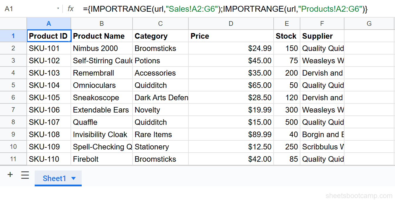
={IMPORTRANGE("https://docs.google.com/spreadsheets/d/SOURCE_ID/edit","Sales!A2:G10");IMPORTRANGE("https://docs.google.com/spreadsheets/d/SOURCE_ID/edit","Inventory!A2:F5")}

The semicolon between the two IMPORTRANGE formulas stacks them vertically — the Inventory rows appear directly below the Sales rows.

Notice the ranges start at row 2, not row 1. This skips the header rows from both tabs, so you get one clean dataset without duplicate headers in the middle.

The column count requirement is the main limitation of this approach. If your two tabs have different structures, stacking with curly braces won’t work cleanly. In that case, keep them as separate imports or use QUERY to reshape the data before combining.

Combining IMPORTRANGE with QUERY

QUERY gives you more control over what data you import. You can filter rows, exclude blanks, reorder columns, or label the output.

Filter out blank rows after stacking:

=QUERY({IMPORTRANGE("https://docs.google.com/spreadsheets/d/SOURCE_ID/edit","Sales!A2:G10");IMPORTRANGE("https://docs.google.com/spreadsheets/d/SOURCE_ID/edit","Inventory!A2:G10")},"SELECT * WHERE Col1 IS NOT NULL")

Stacked ranges sometimes produce blank rows at the bottom when the imported data doesn’t fill the full range. WHERE Col1 IS NOT NULL removes them.

Import from one tab and filter rows:

=QUERY(IMPORTRANGE("https://docs.google.com/spreadsheets/d/SOURCE_ID/edit","Sales!A1:G10"),"SELECT * WHERE Col7 = 'West'",1)

This pulls only the rows where the Region column (Col7) equals “West”. The third argument, 1, tells QUERY how many header rows the imported data has.

Import from one tab and select specific columns:

=QUERY(IMPORTRANGE("https://docs.google.com/spreadsheets/d/SOURCE_ID/edit","Sales!A1:G10"),"SELECT Col1, Col3, Col5, Col6",1)

This returns only Date, SKU, Unit Price, and Total — skipping columns you don’t need in the destination.

For a deeper look at QUERY syntax, see the QUERY function guide.

Common Errors

#REF! with “Unable to parse range”

The tab name in your formula doesn’t match the actual tab name in the source spreadsheet. Open the source file, right-click the tab, and copy the exact name. Paste it into your formula. Watch for trailing spaces in the tab name — they cause this error and are invisible.

#REF! with “You need to connect these sheets”

The Allow access prompt has not been clicked. Hover over the error cell in the destination spreadsheet and click the Allow access button in the popup. If you don’t see the button, try reloading the destination spreadsheet.

Error when stacking with curly braces

The two ranges have different column counts. Count the columns in each range string. Both must match exactly. If Sales!A2:G10 is 7 columns, Inventory!A2:G10 must also reference 7 columns — even if the Inventory tab only has data in 6 of them.

QUERY errors with “Col” references

When you use QUERY on an IMPORTRANGE result, columns are referenced as Col1, Col2, Col3 — not by their letter names (A, B, C). This is because IMPORTRANGE returns an array, not a named spreadsheet range. Replace any column letter references with Col number references.

Tips and Best Practices

1. Name your ranges in the source spreadsheet. Go to Data > Named ranges in the source file and create named ranges for each tab’s data. Then reference the name in IMPORTRANGE: "MyNamedRange" instead of "Sales!A1:G10". Named ranges update automatically if you add rows, so your import doesn’t go stale.

2. Use a helper sheet for imported data. Instead of using IMPORTRANGE directly in your analysis formulas, import the data onto a dedicated helper sheet first. Then run your VLOOKUP, QUERY, or pivot logic against the local copy. This reduces the number of live external connections and makes the spreadsheet faster.

3. Avoid importing entire columns. "Sales!A:G" works, but it imports every row in those columns — including thousands of empty rows. Use explicit row numbers like "Sales!A1:G500" to limit the import size.

4. Keep the source URL as a named cell reference. Put the source spreadsheet URL in a cell (say, B1) and reference it in your IMPORTRANGE formulas: =IMPORTRANGE(B1, "Sales!A1:G10"). If the source URL ever changes, you update one cell instead of every formula.

5. Test tab names before writing complex formulas. Enter a minimal IMPORTRANGE first: =IMPORTRANGE(url, "TabName!A1"). If it returns a value, the tab name is correct. Then build out the full range and any stacking or QUERY logic on top.

Related Google Sheets Tutorials

• IMPORTRANGE in Google Sheets — Full guide to the syntax, access model, and common use cases
• Fix IMPORTRANGE Access Permission - How to grant, manage, and revoke spreadsheet connections
• VLOOKUP with IMPORTRANGE - Look up values from an external spreadsheet
• QUERY Function in Google Sheets - Filter, sort, and reshape data with SQL-style syntax
• IMPORTRANGE with FILTER - Filter imported data without QUERY

Frequently Asked Questions

Can IMPORTRANGE pull from multiple tabs at once?

Not in a single IMPORTRANGE call. Each IMPORTRANGE references one tab. To combine data from multiple tabs, use curly braces to stack results: ={IMPORTRANGE(url,"Sales!A1:G10");IMPORTRANGE(url,"Inventory!A1:G10")}. Both ranges must have the same number of columns.

How do I specify a tab name in IMPORTRANGE?

Include the tab name before the exclamation mark in the range string: "TabName!A1:D10". If the tab name contains spaces, write them as-is: "Sales Data!A1:D10". The quotes around the full range_string handle it.

What happens if I misspell the tab name in IMPORTRANGE?

IMPORTRANGE returns a #REF! error with the message “Unable to parse range.” Double-check that the tab name in your formula matches the tab name in the source spreadsheet exactly, including capitalization.

Can I use QUERY with IMPORTRANGE from multiple tabs?

Yes. Wrap the stacked IMPORTRANGE in QUERY: =QUERY({IMPORTRANGE(url,"Sales!A1:G10");IMPORTRANGE(url,"Inventory!A1:G10")},"SELECT * WHERE Col1 IS NOT NULL"). This filters out blank rows that sometimes appear between the stacked ranges.

Do I need to grant access for each tab separately?

No. Access is granted once per source-destination spreadsheet pair, not per tab. After you click Allow access for the first IMPORTRANGE formula pointing to a source file, all other IMPORTRANGE formulas referencing different tabs in that same file work automatically.