VLOOKUP with IMPORTRANGE in Google Sheets
Combine VLOOKUP with IMPORTRANGE to look up values from another Google Sheets spreadsheet. Step-by-step formula guide with examples and performance tips.
Sheets Bootcamp
March 11, 2026
VLOOKUP searches for a value within the current spreadsheet. IMPORTRANGE pulls data from an external spreadsheet. Combining the two lets you look up values from a completely different Google Sheets file — no copy-pasting required.
This guide covers the combined formula syntax, a step-by-step example with product data, and a performance pattern that keeps your spreadsheet fast.
In This Guide
- How VLOOKUP + IMPORTRANGE Works
- VLOOKUP with IMPORTRANGE: Step-by-Step
- Practical Examples
- The Helper Range Pattern
- Common Errors
- Tips
- Related Google Sheets Tutorials
- Frequently Asked Questions
How VLOOKUP + IMPORTRANGE Works
VLOOKUP takes a range as its second argument — the table to search. Normally, this is a range on the current sheet like A2:D10. When you replace that range with an IMPORTRANGE call, VLOOKUP searches data from an external spreadsheet instead.
=VLOOKUP(lookup_value, IMPORTRANGE("spreadsheet_url", "Sheet!Range"), column_index, FALSE)| Part | What It Does |
|---|---|
lookup_value | The value to search for (e.g., a product ID in cell A2) |
IMPORTRANGE(...) | Fetches the lookup table from an external spreadsheet |
column_index | Which column in the imported table to return |
FALSE | Exact match (use this in most cases) |
The IMPORTRANGE call runs first, pulling the external data into memory. VLOOKUP then searches that data as if it were a local range.
The first time you use IMPORTRANGE with a new source spreadsheet, you need to grant access. See the IMPORTRANGE access permission guide for details.
VLOOKUP with IMPORTRANGE: Step-by-Step
We’ll look up product prices from an external “Product Inventory” spreadsheet. The source has a Products tab with Product ID, Product Name, Category, and Price in columns A through D.
Source Data (External Spreadsheet)
The external spreadsheet holds the product inventory:
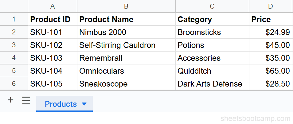
Identify the source data
Open the external spreadsheet and note:
- Spreadsheet URL — copy from the address bar
- Tab name — “Products”
- Range — A2:D6 (skip the header row so VLOOKUP matches data rows directly)
The lookup column (Product ID) is in column A, which is the first column of the range. VLOOKUP requires the search column to be the leftmost column.
Enter the VLOOKUP + IMPORTRANGE formula
In your destination spreadsheet, column A has product IDs you want to look up. Select cell B2 and enter:
=VLOOKUP(A2, IMPORTRANGE("https://docs.google.com/spreadsheets/d/abc123/edit", "Products!A2:D6"), 4, FALSE)Here is what each part does:
A2— the Product ID to look up (SKU-101)IMPORTRANGE(...)— fetches rows 2-6 from the Products tab in the external file4— return the value from column 4 (Price)FALSE— exact match only
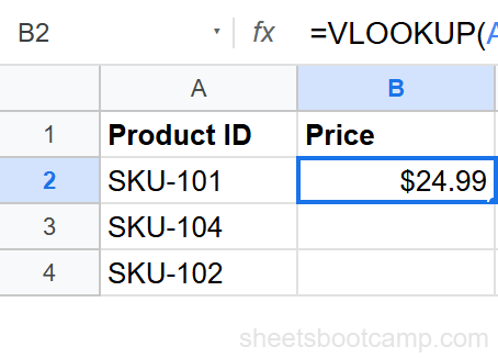
Grant access when prompted
The cell shows a #REF! error. This is the standard IMPORTRANGE access prompt. Hover over the cell and click Allow access in the tooltip.
You only need to do this once. After granting access, every IMPORTRANGE formula between these two spreadsheets works without another prompt.
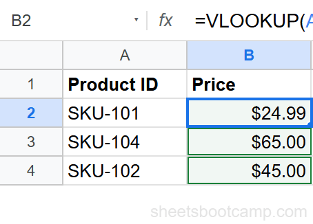
Verify the result
The formula returns $24.99, the price for SKU-101, pulled from the external Products spreadsheet. Copy the formula down to B3 and B4. SKU-104 returns $65.00 and SKU-102 returns $45.00.
Use the spreadsheet ID instead of the full URL for a shorter formula. The ID is the string between /d/ and /edit in the URL. The formula works the same with either format.
Practical Examples
Example 1: Dynamic Lookup from a Cell Reference
Instead of hardcoding the lookup value, reference a cell. This is the standard pattern for real spreadsheets:
=VLOOKUP(A2, IMPORTRANGE("https://docs.google.com/spreadsheets/d/abc123/edit", "Products!A2:D6"), 4, FALSE)When you change the value in A2, the VLOOKUP automatically searches the external spreadsheet for the new value. Copy the formula down the column, and each row looks up its own Product ID.
Example 2: Return a Different Column
Change the column index to return a different field. To get the product name (column 2) instead of the price (column 4):
=VLOOKUP(A2, IMPORTRANGE("https://docs.google.com/spreadsheets/d/abc123/edit", "Products!A2:D6"), 2, FALSE)This returns “Nimbus 2000” for SKU-101. The column index counts from the first column of the imported range, not from column A.
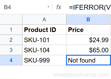
Example 3: IFERROR for Clean Error Handling
When a product ID does not exist in the external table, VLOOKUP returns #N/A. Wrap the formula in IFERROR to show a readable message instead:
=IFERROR(VLOOKUP(A4, IMPORTRANGE("https://docs.google.com/spreadsheets/d/abc123/edit", "Products!A2:D6"), 4, FALSE), "Not found")For SKU-999 (which does not exist in the source), this returns “Not found” instead of #N/A. For valid IDs, the price appears as normal.
IFERROR catches all errors, including #REF! from access issues. If you want to distinguish between “not found” and “access not granted,” check the IMPORTRANGE access permission guide before adding IFERROR.
The Helper Range Pattern
When multiple rows use VLOOKUP + IMPORTRANGE, each row makes a separate call to the external spreadsheet. With 50 rows, that is 50 IMPORTRANGE calls, and the spreadsheet slows down noticeably.
The fix: import the external data once into a helper range, then VLOOKUP against the local copy.
Step 1: In an unused area (or a hidden sheet), enter the IMPORTRANGE formula once:
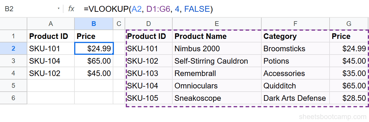
=IMPORTRANGE("https://docs.google.com/spreadsheets/d/abc123/edit", "Products!A1:D6")This imports the full product table into cells D1:G6 (or wherever you place it).
Step 2: Write your VLOOKUP against the local helper range:
=VLOOKUP(A2, D1:G6, 4, FALSE)Now the lookup runs against local data. One IMPORTRANGE call, unlimited VLOOKUP formulas.
The helper range pattern is the recommended approach when you have more than 5-10 VLOOKUP + IMPORTRANGE formulas. The spreadsheet stays responsive, and updating the source data still propagates automatically through the single IMPORTRANGE call.
Common Errors
#REF! Error: Access Not Granted
The most common error with this formula. The IMPORTRANGE part has not been authorized.
Fix: Hover over the error cell and click Allow access. If the popup does not appear, check that the URL and range string are correct. See the access permission guide for more troubleshooting.
#N/A Error: Value Not Found
The VLOOKUP part cannot find the lookup value in the first column of the imported data. This works the same as a regular VLOOKUP #N/A error. Common causes:
- Extra spaces in the lookup value or the source data
- Different data types (text “101” vs number 101)
- The value genuinely does not exist in the source
Fix: Use =TRIM(A2) to clean whitespace. Verify the value exists in the external spreadsheet.
#VALUE! Error: Bad URL or Range
The IMPORTRANGE URL is malformed, or the range string does not match a valid sheet and range in the source.
Fix: Open the source spreadsheet, copy the URL directly from the address bar, and verify the sheet tab name and range.
Formula Is Slow
Each VLOOKUP + IMPORTRANGE call fetches data from the external file independently. With many rows, this adds up.
Fix: Use the helper range pattern. Import the data once, then VLOOKUP against the local copy.
Tips
-
Use the helper range pattern for more than 5-10 lookups. One IMPORTRANGE call is faster than 50 individual ones. Import the table into a hidden sheet and VLOOKUP against it.
-
Include the header row in the helper range but not in the VLOOKUP range. Import
A1:D100into the helper area so you can see column labels. But set the VLOOKUP range to start at the data rows (skip the header) so the header is not treated as a match. -
Use IFERROR for user-facing spreadsheets.
=IFERROR(VLOOKUP(...), "Not found")keeps the output clean when a lookup value is missing from the source. -
Use absolute references in the IMPORTRANGE range string. The range string like
"Products!A2:D6"does not use cell references, so it does not shift when copied. But your VLOOKUP lookup_value (A2) should use relative references so it adjusts per row. -
Grant IMPORTRANGE access proactively. Before sharing the destination spreadsheet, enter the formula and click “Allow access” yourself. Your colleagues won’t encounter the #REF! prompt.
Related Google Sheets Tutorials
- IMPORTRANGE: The Complete Guide — Full syntax, access permissions, and combining with other functions
- Fix IMPORTRANGE Access Permission — Troubleshoot the “You need to connect these sheets” error
- VLOOKUP: The Complete Guide — VLOOKUP fundamentals before combining with IMPORTRANGE
- VLOOKUP from Another Sheet — Cross-tab VLOOKUP within the same spreadsheet (not cross-file)
- Fix VLOOKUP Errors — Troubleshoot #N/A, #REF!, and #VALUE! errors
Frequently Asked Questions
Can VLOOKUP pull data from another spreadsheet?
Not on its own. VLOOKUP searches within the current spreadsheet. To look up values from a different spreadsheet file, use IMPORTRANGE as the table_array argument: =VLOOKUP(A2, IMPORTRANGE(“url”, “Sheet1!A2:D10”), 4, FALSE).
Why does VLOOKUP with IMPORTRANGE show #REF?
The #REF! error usually means access has not been granted. Hover over the error cell and click Allow access. If the error persists, check that the URL and range string in the IMPORTRANGE part are correct.
Is VLOOKUP with IMPORTRANGE slow?
It can be. IMPORTRANGE fetches data from the external spreadsheet on every recalculation. For better performance, import the external data into a helper range first, then run VLOOKUP against the local copy.
Can I use INDEX MATCH with IMPORTRANGE instead?
Yes. INDEX MATCH works with IMPORTRANGE the same way: =INDEX(IMPORTRANGE(“url”, “Sheet1!D2:D10”), MATCH(A2, IMPORTRANGE(“url”, “Sheet1!A2:A10”), 0)). This requires two IMPORTRANGE calls, which may be slower than the VLOOKUP approach.
Do I need to grant access every time I use this formula?
No. Access is granted once per source-destination spreadsheet pair. After the first Allow access click, all IMPORTRANGE formulas between those two files work without another prompt.