INDEX MATCH in Google Sheets: Complete Guide
Learn how to use INDEX MATCH in Google Sheets to look up values in any direction. Covers syntax, left lookups, multiple criteria, and common error fixes.
Sheets Bootcamp
February 18, 2026
INDEX MATCH in Google Sheets combines two functions — INDEX and MATCH — to look up values from any column in your data, regardless of direction. Unlike VLOOKUP, which only searches the leftmost column and returns values to the right, INDEX MATCH can look left, right, or across both rows and columns.
This guide covers the syntax of both functions, walks through combining them step by step, and shows practical examples including left lookups, two-way lookups, and multiple criteria matching.
In This Guide
- What Is INDEX MATCH?
- INDEX Function Syntax
- MATCH Function Syntax
- The Combined INDEX MATCH Formula
- How to Use INDEX MATCH: Step-by-Step
- INDEX MATCH Examples
- INDEX MATCH vs VLOOKUP
- Common Errors and How to Fix Them
- Tips and Best Practices
- Related Google Sheets Tutorials
- FAQ
What Is INDEX MATCH?
INDEX MATCH is a two-function lookup pattern in Google Sheets. MATCH finds the position of a value in a column (or row), and INDEX returns the value at that position from a different column (or row). The two functions were designed independently, but combining them creates a lookup formula that is more flexible than VLOOKUP.
The main advantages of INDEX MATCH:
- Any direction — look up values to the left, right, or in a completely different part of the sheet
- Column-insertion safe — adding or removing columns between your lookup and return ranges does not break the formula
- Multiple criteria — match on two or more conditions using array formulas
- Two-way lookups — find a value at the intersection of a specific row and column
INDEX MATCH has a steeper learning curve than VLOOKUP. The formula uses two functions instead of one, and you need to understand how the row position from MATCH feeds into INDEX. But once you understand how the two pieces fit together, you can handle lookups that VLOOKUP cannot.
Google Sheets also supports XLOOKUP, which was designed to replace both VLOOKUP and INDEX MATCH with a single function. INDEX MATCH remains relevant because it offers array-based multiple criteria matching and two-way lookups that XLOOKUP does not support natively.
INDEX Function Syntax
INDEX returns a value from a range based on a row number (and optionally a column number).
=INDEX(reference, row, [column])| Parameter | Description | Required |
|---|---|---|
| reference | The range of cells to return a value from | Yes |
| row | The row number within the range (1 = first row) | Yes |
| column | The column number within the range (1 = first column). Defaults to 1 for single-column ranges | No |
A quick example using the product inventory data:
=INDEX(D2:D9, 3)This returns $35.00 — the value in the 3rd row of D2:D9, which is cell D4 (the Remembrall’s price).
INDEX counts rows starting at 1 within the range you provide, not from the top of the sheet. If your range is D2:D9, row 1 is D2, row 2 is D3, and so on.
MATCH Function Syntax
MATCH searches for a value in a single row or column and returns its position (as a number).
=MATCH(search_key, range, [match_type])| Parameter | Description | Required |
|---|---|---|
| search_key | The value to search for | Yes |
| range | A single row or column to search within | Yes |
| match_type | 0 for exact match, 1 for less than or equal (sorted ascending), -1 for greater than or equal (sorted descending). Defaults to 1 | No |
A quick example:
=MATCH("SKU-103", A2:A9, 0)This returns 3 because “SKU-103” is the 3rd value in the range A2:A9. Note that MATCH returns the position within the range, not the row number of the sheet. A2 is position 1, A3 is position 2, and A4 is position 3.
Always set match_type to 0 for exact matching. The default is 1, which assumes your data is sorted in ascending order and returns the closest match less than or equal to the search key. On unsorted data, 1 returns wrong results without any error message.
MATCH is not case-sensitive. =MATCH("sku-103", A2:A9, 0) returns the same result as =MATCH("SKU-103", A2:A9, 0). If you need case-sensitive matching, see the tip in the Best Practices section below.
The Combined INDEX MATCH Formula
The core INDEX MATCH pattern nests MATCH inside the row argument of INDEX:
=INDEX(return_range, MATCH(search_key, lookup_range, 0))Here is the logic:
- MATCH searches for
search_keyinlookup_rangeand returns its row position - INDEX takes that position and returns the corresponding value from
return_range
The key requirement: return_range and lookup_range must have the same number of rows (and start from the same row) so the position numbers line up.
Using the product inventory data to find the price for SKU-103:
=INDEX(D2:D9, MATCH("SKU-103", A2:A9, 0))- MATCH finds “SKU-103” at position 3 in A2:A9
- INDEX returns the 3rd value from D2:D9, which is $35.00
Think of it this way: MATCH answers “which row?” and INDEX answers “what value is in that row?” Neither function is useful on its own for lookups, but together they form a complete lookup system.
How to Use INDEX MATCH: Step-by-Step
We’ll build an INDEX MATCH formula from scratch using a product inventory table. The goal: look up a Product ID and return its price.
Sample Data
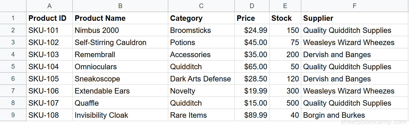
Set up your data
You need a table with at least two columns — one to search in and one to return values from. This product inventory has Product IDs in column A and Prices in column D. The data runs from row 2 to row 9 (8 products).
Write the MATCH formula
First, find the position of the Product ID you are looking for. Select an empty cell and enter:
=MATCH("SKU-103", A2:A9, 0)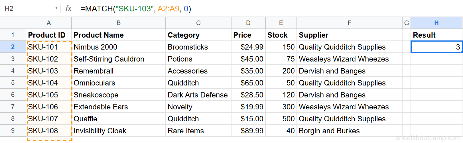
This returns 3 because “SKU-103” (the Remembrall) is the 3rd entry in A2:A9. The 0 at the end means exact match.
Write the INDEX formula
Now use that position to pull the price. In another cell, enter:
=INDEX(D2:D9, 3)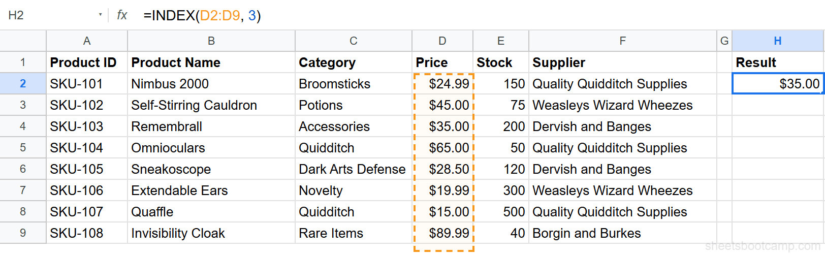
This returns $35.00 — the 3rd value in the Price column (D2:D9).
Combine INDEX and MATCH
Replace the hardcoded 3 with the MATCH function:
=INDEX(D2:D9, MATCH("SKU-103", A2:A9, 0))
The formula returns $35.00. MATCH finds the position, INDEX pulls the value — all in one formula.
Make it dynamic with a cell reference
Replace the hardcoded search key with a cell reference so you can look up any product:
=INDEX(D2:D9, MATCH(H2, A2:A9, 0))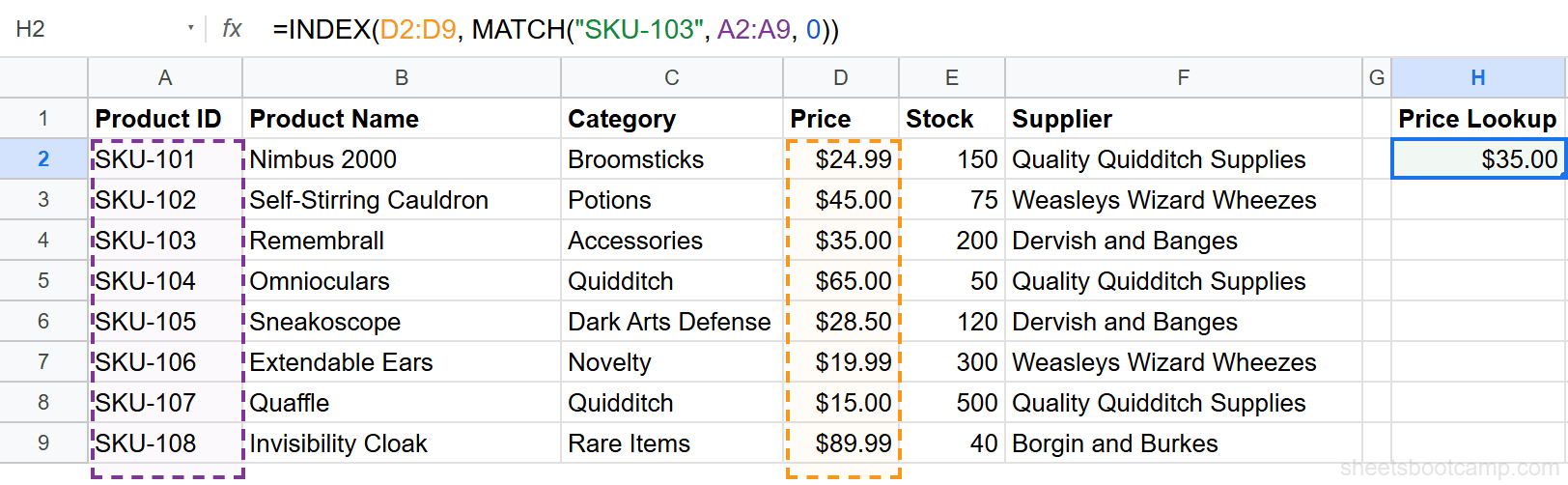
Type any Product ID in cell H2, and the formula returns the matching price. Enter “SKU-108” and it returns $89.99 (the Invisibility Cloak). Change it to “SKU-106” and the result updates to $19.99 (Extendable Ears).
When copying INDEX MATCH formulas down a column, lock the lookup and return ranges with absolute references: =INDEX($D$2:$D$9, MATCH(H2, $A$2:$A$9, 0)). The search key reference (H2) should stay relative so it shifts with each row.
INDEX MATCH Examples
Example 1: Left Lookup
VLOOKUP requires the search column to be the leftmost column in your range. INDEX MATCH has no such restriction.
You want to find the Product ID (column A) for a product named “Remembrall” (column B). Since the Product Name is to the right of the Product ID, VLOOKUP cannot do this.
=INDEX(A2:A9, MATCH("Remembrall", B2:B9, 0))- MATCH finds “Remembrall” at position 3 in B2:B9
- INDEX returns the 3rd value from A2:A9, which is “SKU-103”
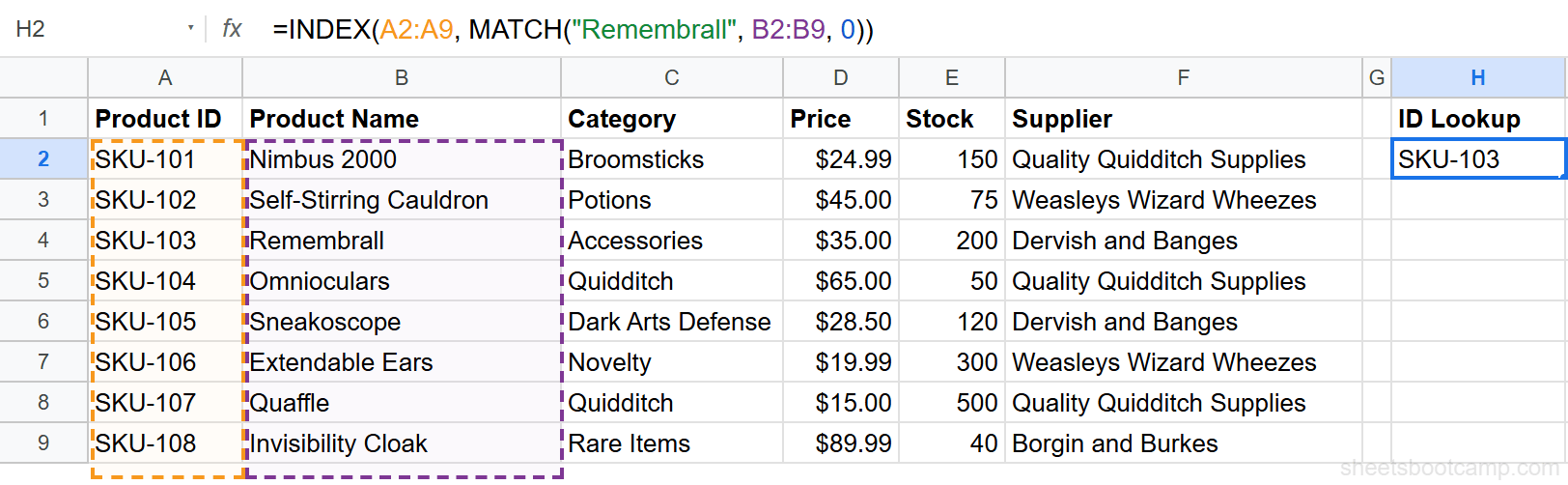
This is the classic INDEX MATCH advantage over VLOOKUP. To do this with VLOOKUP, you would need to rearrange your data so the Product Name column comes before the Product ID column — or add a helper column. INDEX MATCH handles it without changing your data structure at all.
For more patterns and edge cases, see the full guide on left lookups with INDEX MATCH.
Example 2: Two-Way Lookup
A two-way lookup finds a value at the intersection of a specific row and column. Use MATCH twice — once for the row and once for the column.
You want to find the Stock value for SKU-104. Instead of hardcoding the column position, use MATCH to find the “Stock” column by searching the header row.
=INDEX(A2:F9, MATCH("SKU-104", A2:A9, 0), MATCH("Stock", A1:F1, 0))- The first MATCH finds “SKU-104” at row position 4 in A2:A9
- The second MATCH finds “Stock” at column position 5 in A1:F1
- INDEX returns the value at row 4, column 5 of A2:F9, which is 50
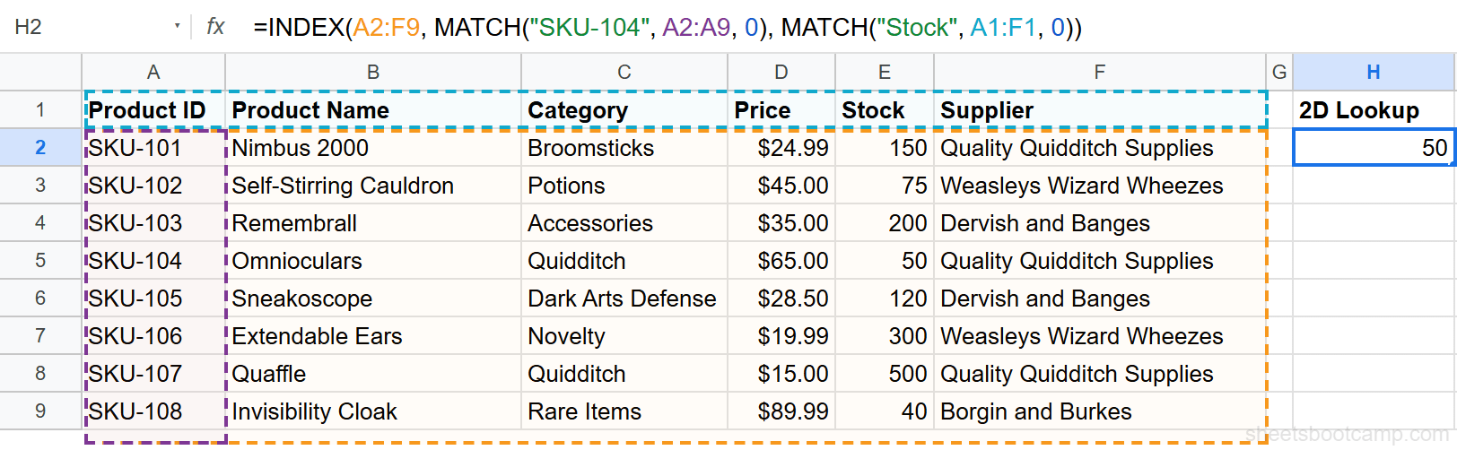
This approach is column-insertion safe. If you add a new column between Price and Stock, the second MATCH still finds “Stock” at the correct position. Two-way lookups are useful when your data has many columns and you want to select the return column dynamically — for example, by picking a column header from a dropdown list created with data validation.
For more two-way lookup patterns, see two-way lookups with INDEX MATCH.
Example 3: Multiple Criteria Lookup
Standard INDEX MATCH handles one search criterion. To match on two or more conditions, multiply them inside MATCH and search for 1.
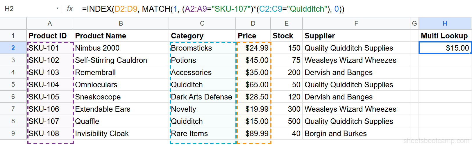
You want to find the price for a product that is both SKU-107 AND in the “Quidditch” category:
=INDEX(D2:D9, MATCH(1, (A2:A9="SKU-107")*(C2:C9="Quidditch"), 0))(A2:A9="SKU-107")returns an array of TRUE/FALSE values(C2:C9="Quidditch")returns another array of TRUE/FALSE values- Multiplying them together gives 1 only where both conditions are true
- MATCH finds the first
1in the resulting array, which points to the Quaffle - INDEX returns $15.00 from column D
In current versions of Google Sheets, this formula works with a standard Enter press. In older versions, you may need to press Ctrl+Shift+Enter to enter it as an array formula. If the formula returns an error, try the Ctrl+Shift+Enter approach.
For more multi-criteria patterns, see the full guide on INDEX MATCH with multiple criteria.
INDEX MATCH vs VLOOKUP
Both formulas look up values in a table, but they differ in flexibility and behavior.
| Feature | VLOOKUP | INDEX MATCH |
|---|---|---|
| Lookup direction | Right only (search key must be in the leftmost column) | Any direction |
| Column insertions | Breaks the formula (column index number shifts) | Safe (references specific ranges) |
| Performance on large data | Slightly faster for single lookups | Comparable in most cases |
| Learning curve | Easier to write and read | Steeper, requires understanding two functions |
| Return column flexibility | Uses a column index number (e.g., 3 for 3rd column) | References the return range directly |
| Multiple criteria | Requires a helper column or ARRAYFORMULA workaround | Built-in with array multiplication |
| Two-way lookups | Not possible without nesting | Supported with dual MATCH |
When to use VLOOKUP: Your search column is the leftmost column, you have a stable table structure, and the formula needs to be readable by other team members. VLOOKUP communicates its purpose in a single function call, which makes it faster to audit.
When to use INDEX MATCH: Your search column is not the leftmost, you expect columns to be added or removed, you need multiple criteria, or you need a two-way lookup. INDEX MATCH is also the better choice in shared spreadsheets where other people regularly add or rearrange columns. A VLOOKUP formula that references column 4 will break — or worse, silently return the wrong column — after someone inserts a new column. INDEX MATCH references the return range directly, so column changes do not affect it.
A Practical Example of the Difference
Consider looking up the Supplier for SKU-105 in the product inventory. With VLOOKUP:
=VLOOKUP("SKU-105", A2:F9, 6, FALSE)This works because Supplier is the 6th column. But if someone inserts a “Discount” column between Price and Stock, Supplier moves to column 7. The VLOOKUP formula still says 6, and now it returns the Stock value (120) instead of the Supplier name. No error appears.
With INDEX MATCH:
=INDEX(F2:F9, MATCH("SKU-105", A2:A9, 0))This formula references column F directly. If a new column is inserted before F, Google Sheets automatically updates the reference to G2:G9. The formula continues to return “Dervish and Banges” regardless of structural changes.
For a detailed side-by-side comparison with more examples, see INDEX MATCH vs VLOOKUP.
Common Errors and How to Fix Them
#N/A Error
MATCH could not find the search key in the lookup range. This is the most common INDEX MATCH error.
Common causes:
- Typos or extra spaces — “SKU-103 ” (with a trailing space) does not match “SKU-103”
- Mismatched data types — searching for the number 103 in a column of text values like “SKU-103”
- Wrong range — the lookup range does not include the row containing your search key
To check for extra spaces, use =LEN(A2) to see the character count. If “SKU-103” shows a length of 8 instead of 7, there is a hidden space. Clean the data with =TRIM(A2).
To handle the error gracefully, wrap the entire formula in IFERROR:
=IFERROR(INDEX(D2:D9, MATCH("SKU-103", A2:A9, 0)), "Not found")This returns “Not found” instead of #N/A when the lookup fails.
Use =IFERROR(INDEX(..., MATCH(..., ..., 0)), "") with an empty string to display a blank cell instead of an error message. This keeps your spreadsheet clean when lookups are expected to fail for some rows.
#REF! Error
The row number returned by MATCH exceeds the number of rows in the INDEX range. This happens when the two ranges have different sizes.
For example, if MATCH searches A2:A9 (8 rows) but INDEX references D2:D5 (4 rows), a match at position 5 or higher causes #REF! because INDEX cannot return row 5 from a 4-row range.
Fix: make sure both ranges have the same number of rows. A2:A9 and D2:D9 both cover 8 rows. A common cause is accidentally including the header row in one range but not the other — A1:A9 has 9 rows while D2:D9 has 8.
#VALUE! Error
The match_type argument in MATCH is not a valid value. It must be 0, 1, or -1. Any other value returns #VALUE!.
This also happens if the lookup range in MATCH contains more than one row and more than one column. MATCH works on a single row or a single column, not a 2D range. For example, =MATCH("SKU-103", A2:B9, 0) returns #VALUE! because A2:B9 spans two columns. Use A2:A9 (one column) instead.
Wrong Result (No Error)
If your formula returns a value but it is the wrong one, check the match_type argument. Using 1 (the default) on unsorted data causes MATCH to return incorrect positions without any error.
MATCH with match_type set to 1 or -1 requires sorted data. On unsorted data, it returns wrong positions silently — no error message appears. Always use 0 for exact matching unless your data is specifically sorted for approximate matching.
Tips and Best Practices
-
Always use 0 as the third argument in MATCH. The default (
1) assumes sorted data and performs approximate matching. For exact lookups,0is the correct choice. -
Lock your ranges with absolute references. When copying INDEX MATCH formulas to multiple rows, use
$signs on the ranges:=INDEX($D$2:$D$9, MATCH(H2, $A$2:$A$9, 0)). The search key cell (H2) stays relative. -
Wrap in IFERROR for clean error handling.
=IFERROR(INDEX(..., MATCH(..., ..., 0)), "Not found")returns a custom message instead of #N/A when the lookup fails. -
Use INDEX MATCH when the lookup column is not the leftmost. VLOOKUP requires the search key in the first column of the range. INDEX MATCH has no such requirement — set the MATCH range to any column.
-
For case-sensitive lookups, combine MATCH with EXACT. Standard MATCH is not case-sensitive. To match “sku-103” differently from “SKU-103”, use an array formula:
=INDEX(D2:D9, MATCH(TRUE, EXACT(A2:A9, "sku-103"), 0)). -
Name your ranges for readability. Instead of
=INDEX(D2:D9, MATCH(H2, A2:A9, 0)), define named ranges (Data > Named ranges) likePricesfor D2:D9 andProductIDsfor A2:A9. The formula becomes=INDEX(Prices, MATCH(H2, ProductIDs, 0)), which is easier to read and maintain.
If you find yourself writing the same INDEX MATCH formula in multiple cells with different return columns, consider whether a QUERY function could replace them. A single QUERY formula can return multiple columns at once.
Related Google Sheets Tutorials
- INDEX MATCH Basics — A beginner-friendly walkthrough of how INDEX and MATCH work together
- INDEX MATCH vs VLOOKUP — Detailed comparison with benchmarks and migration tips
- INDEX MATCH with Multiple Criteria — Match on two or more conditions using array formulas
- Left Lookups with INDEX MATCH — Return values from columns to the left of your search column
- VLOOKUP in Google Sheets — The simpler lookup function, best for standard right-to-left lookups
- QUERY Function Guide — Filter, sort, and summarize data with SQL-like syntax in a single formula
Frequently Asked Questions
What is INDEX MATCH in Google Sheets?
INDEX MATCH combines two functions to look up data. MATCH finds the row position of a value, and INDEX returns the value at that position from a different column. Together they work like VLOOKUP but can look in any direction.
Is INDEX MATCH better than VLOOKUP?
INDEX MATCH is more flexible. It can look left, handles column insertions without breaking, and supports multiple criteria with array formulas. VLOOKUP is easier to learn and works well for standard right-to-left lookups.
How do I use INDEX MATCH to look left?
Set the INDEX range to the column on the left and the MATCH range to a column on the right. For example, =INDEX(A2:A9, MATCH("Remembrall", B2:B9, 0)) returns the Product ID from column A by searching Product Name in column B.
Can INDEX MATCH handle multiple criteria?
Yes. Multiply conditions inside MATCH and search for 1: =INDEX(D2:D9, MATCH(1, (A2:A9="SKU-107")*(C2:C9="Quidditch"), 0)). In current versions of Google Sheets, press Enter. In older versions, press Ctrl+Shift+Enter.
Why does INDEX MATCH return #N/A?
The #N/A error means MATCH could not find the search key in the lookup range. Check for typos, extra spaces, or mismatched data types (text vs. number). Also confirm the third argument in MATCH is set to 0 for exact matching.
Do I need Ctrl+Shift+Enter for INDEX MATCH?
Only for array formulas like multiple criteria lookups. Standard INDEX MATCH formulas work with regular Enter. Current versions of Google Sheets handle most array formulas automatically without Ctrl+Shift+Enter.
Can INDEX MATCH return values from multiple columns?
Not in a single formula, but you can write separate INDEX MATCH formulas pointing to different return columns. Each formula uses the same MATCH logic but changes the INDEX range. For example, one returns column D (Price) and another returns column E (Stock).