INDEX MATCH for Beginners in Google Sheets
Learn INDEX MATCH in Google Sheets with this beginner tutorial. Step-by-step guide covering MATCH positions, INDEX returns, and combining both functions.
Sheets Bootcamp
March 12, 2026
INDEX MATCH in Google Sheets combines two functions to look up values from any column in your data. MATCH finds the row position of the value you are searching for, and INDEX returns the data at that position from a different column. This tutorial walks through each function separately, then shows how to combine them into a single lookup formula.
In This Guide
- What Is INDEX MATCH?
- How MATCH Works
- How INDEX Works
- Combining INDEX and MATCH: Step-by-Step
- Make INDEX MATCH Dynamic
- Why INDEX MATCH Instead of VLOOKUP?
- Common Mistakes Beginners Make
- Tips for Beginners
- Related Google Sheets Tutorials
- Frequently Asked Questions
What Is INDEX MATCH?
INDEX MATCH is a two-function lookup pattern. MATCH answers “which row is this value in?” and INDEX answers “what value is in that row?” Neither function does a full lookup on its own, but together they form a flexible alternative to VLOOKUP.
The key advantage: INDEX MATCH can return values from any column, including columns to the left of your search column. VLOOKUP can only return values to the right. INDEX MATCH also does not break when you insert or delete columns, because each function references its own specific range.
How MATCH Works
MATCH searches for a value in a single column (or row) and returns its position as a number.
=MATCH(search_key, range, match_type)| Parameter | Description | Required |
|---|---|---|
| search_key | The value to search for | Yes |
| range | A single column or row to search within | Yes |
| match_type | 0 for exact match, 1 for less than or equal, -1 for greater than or equal. Defaults to 1 | No |
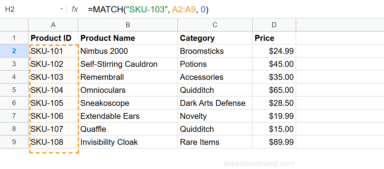
Using the product inventory data, find the position of SKU-103:
=MATCH("SKU-103", A2:A9, 0)This returns 3 because SKU-103 is the 3rd value in the range A2:A9. Position 1 is A2 (SKU-101), position 2 is A3 (SKU-102), and position 3 is A4 (SKU-103).
Always set match_type to 0 for exact matching. The default is 1, which assumes your data is sorted in ascending order and returns approximate matches. On unsorted data, 1 returns wrong results without any error.
MATCH returns a position within the range, not the sheet row number. If your range starts at A2, position 1 corresponds to row 2, position 2 to row 3, and so on.
How INDEX Works
INDEX returns a value from a range based on a row number (and optionally a column number).
=INDEX(range, row_number, [column_number])| Parameter | Description | Required |
|---|---|---|
| range | The range to pull a value from | Yes |
| row_number | Which row within the range (1 = first row) | Yes |
| column_number | Which column within the range (1 = first column). Defaults to 1 for single-column ranges | No |
To get the 3rd price from the Price column:
=INDEX(D2:D9, 3)This returns $35.00 — the 3rd value in D2:D9, which is cell D4 (the Remembrall’s price).
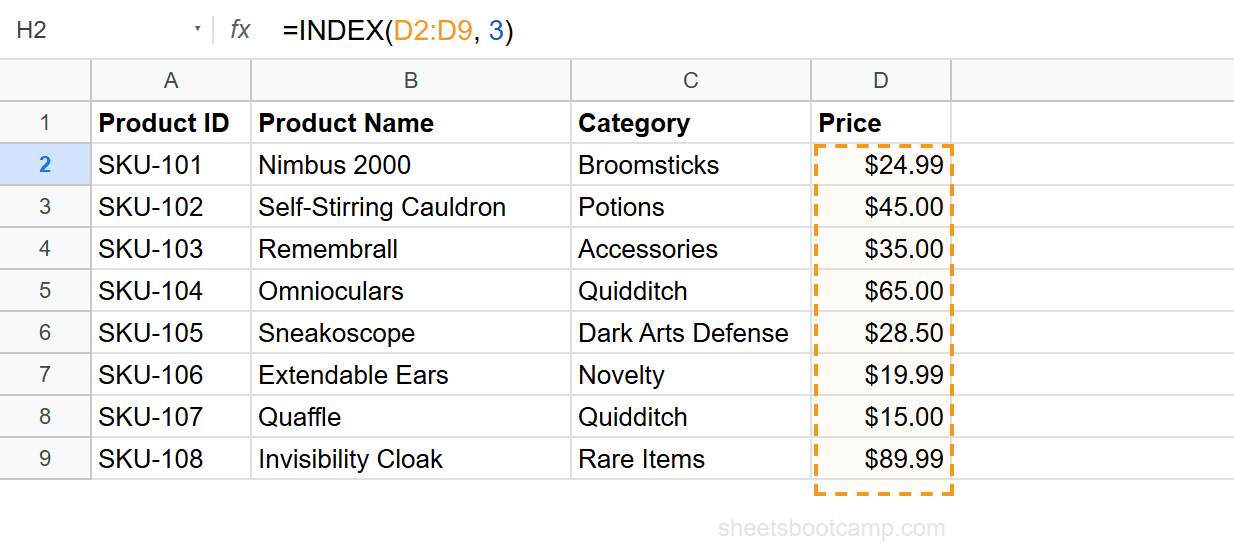
INDEX counts rows starting at 1 within the range you provide. If your range is D2:D9, row 1 is D2, row 2 is D3, row 3 is D4. The numbering is relative to the range, not the sheet.
Combining INDEX and MATCH: Step-by-Step
Now we connect the two functions. MATCH finds the row position, and INDEX uses that position to return a value. The combined formula looks like this:
=INDEX(return_range, MATCH(search_key, lookup_range, 0))We’ll build this step by step using a product inventory table. The goal: look up a Product ID and return its price.
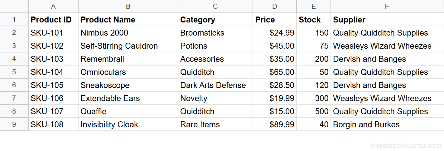
Sample Data
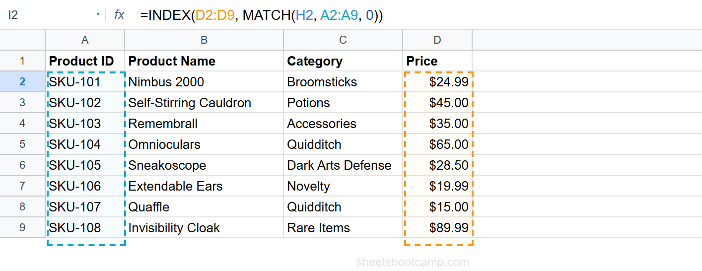
The inventory has Product IDs in column A and Prices in column D, with data in rows 2 through 9 (8 products).
Set up your data
You need a table with at least two columns — one to search in (Product ID) and one to return values from (Price). The product inventory has Product IDs in column A and Prices in column D.
Write the MATCH formula
First, find the position of the Product ID you want. Select an empty cell and enter:
=MATCH("SKU-103", A2:A9, 0)This returns 3 because SKU-103 is the 3rd entry in A2:A9. The 0 means exact match.
Write the INDEX formula
Use the position from MATCH to pull the price. In another cell, enter:
=INDEX(D2:D9, 3)This returns $35.00 — the value at position 3 in the Price column.
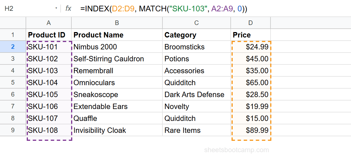
Combine INDEX and MATCH
Replace the hardcoded 3 with the MATCH function:
=INDEX(D2:D9, MATCH("SKU-103", A2:A9, 0))The formula returns $35.00. MATCH finds the position (3), and INDEX pulls the value at that position from the Price column.
Make it dynamic with a cell reference
Replace the hardcoded search key with a cell reference:
=INDEX(D2:D9, MATCH(H2, A2:A9, 0))Type any Product ID in cell H2. Enter SKU-108 and the formula returns $89.99 (the Invisibility Cloak). Change H2 to SKU-106 and the result updates to $19.99 (Extendable Ears).
When copying INDEX MATCH formulas down a column, lock the ranges with absolute references: =INDEX($D$2:$D$9, MATCH(H2, $A$2:$A$9, 0)). The search key reference (H2) stays relative so it shifts per row.
Make INDEX MATCH Dynamic
The dynamic version of INDEX MATCH reads the search key from a cell instead of the formula itself. This is how the formula is used in real spreadsheets.
=INDEX(D2:D9, MATCH(H2, A2:A9, 0))With this pattern, you can:
- Change one cell to update the result — type a different Product ID in H2 and the price updates automatically
- Copy the formula down — if H2:H10 contains different product IDs, copy the formula from I2 to I10 and each row returns its own price
- Build dashboards — combine cell references with data validation dropdowns to let users pick a product from a list
Why INDEX MATCH Instead of VLOOKUP?
If you are new to lookups, you might wonder why INDEX MATCH exists when VLOOKUP does the same thing in a single function. The short answer: INDEX MATCH is more flexible.
VLOOKUP searches the leftmost column only. If you need to return a value from a column to the left of your search column, VLOOKUP cannot do it. INDEX MATCH can, because you set each range independently.
VLOOKUP breaks when columns move. VLOOKUP uses a column index number (e.g., 4 for the 4th column). If someone inserts a column in the middle of your range, that number now points to the wrong column. INDEX MATCH references the return column directly (D2:D9), so column changes do not affect it.
For a full comparison with benchmarks and migration examples, see INDEX MATCH vs VLOOKUP.
Common Mistakes Beginners Make
Mismatched range sizes
The lookup range and return range must have the same number of rows. If MATCH searches A2:A9 (8 rows) but INDEX references D2:D5 (4 rows), a match at position 5 or higher causes a #REF! error.
Fix: Make both ranges the same length. A2:A9 and D2:D9 both cover 8 rows.
Forgetting the 0 in MATCH
MATCH defaults to approximate matching (match_type 1) if you leave out the third argument. On unsorted data, approximate matching returns wrong positions silently.
MATCH with match_type 1 (the default) requires sorted data. On unsorted data, it returns incorrect positions without any error message. Always include 0 for exact matching.
Searching a multi-column range with MATCH
MATCH works on a single column or a single row. Passing a multi-column range like A2:B9 causes a #VALUE! error.
Fix: Narrow the range to one column: A2:A9.
Including headers in the data range
If you include the header row in MATCH’s range (A1:A9 instead of A2:A9), the header takes position 1 and shifts every position by one. This can cause INDEX to return the wrong row.
Fix: Start both ranges at the first data row (row 2), not the header row.
Tips for Beginners
-
Always use 0 as the third argument in MATCH. This ensures exact matching. The default (
1) assumes sorted data and returns approximate matches, which produces wrong results on typical data. -
Lock your ranges with dollar signs. When copying the formula to multiple rows, use
$A$2:$A$9and$D$2:$D$9so the ranges stay fixed. Leave the search key reference (H2) relative. -
Wrap in IFERROR for clean output.
=IFERROR(INDEX(D2:D9, MATCH(H2, A2:A9, 0)), "Not found")shows “Not found” instead of #N/A when the lookup value does not exist. -
Start with MATCH alone. Before writing the full INDEX MATCH formula, test MATCH by itself to confirm it returns the correct position. This makes debugging easier.
-
Think of it as two questions. MATCH asks “where is it?” INDEX asks “what’s there?” Keeping the two questions separate in your head makes the formula intuitive.
Related Google Sheets Tutorials
- INDEX MATCH: The Complete Guide — Full syntax, left lookups, two-way lookups, and multiple criteria matching
- INDEX MATCH vs VLOOKUP — Detailed comparison to help you choose the right function
- INDEX MATCH with Multiple Criteria — Match on two or more conditions using array formulas
- VLOOKUP for Beginners — The simpler lookup function if you are starting from scratch
- VLOOKUP: The Complete Guide — Full VLOOKUP reference with examples and error fixes
Frequently Asked Questions
What does INDEX MATCH do in Google Sheets?
INDEX MATCH looks up a value by combining two functions. MATCH finds the row position of your search key in one column, and INDEX returns the value at that position from a different column. Together they create a flexible lookup.
Is INDEX MATCH harder than VLOOKUP?
INDEX MATCH uses two functions instead of one, so it takes a bit more time to learn. But the pattern is always the same: MATCH finds the row, INDEX pulls the value. Once you see the pattern, it becomes routine.
Do I need to press Ctrl+Shift+Enter for INDEX MATCH?
No. A standard INDEX MATCH formula works with a regular Enter press. Ctrl+Shift+Enter is only needed for advanced array formulas like multiple criteria lookups.
Can INDEX MATCH look left in Google Sheets?
Yes. Unlike VLOOKUP, INDEX MATCH can return values from any column, including columns to the left of your search column. Set the INDEX range to the left column and the MATCH range to the right column.
Why does my INDEX MATCH return #N/A?
The #N/A error means MATCH could not find your search key. Check for typos, extra spaces, and mismatched data types. Also confirm the third argument in MATCH is 0 for exact matching.