Left Lookup with INDEX MATCH in Google Sheets
Use INDEX MATCH for left lookups in Google Sheets. Return values from columns to the left of your search column, something VLOOKUP cannot do.
Sheets Bootcamp
May 7, 2026
A left lookup in Google Sheets returns a value from a column to the left of the column you are searching. VLOOKUP cannot do this because it only searches the leftmost column and returns values to the right. INDEX MATCH handles left lookups by letting you set the return column and search column independently.
In This Guide
- Why VLOOKUP Cannot Look Left
- How INDEX MATCH Solves Left Lookups
- Left Lookup: Step-by-Step
- Practical Examples
- XLOOKUP Alternative
- Tips
- Related Google Sheets Tutorials
- Frequently Asked Questions
Why VLOOKUP Cannot Look Left
VLOOKUP searches the first column of the range you specify and returns a value from a numbered column to the right. The column index (the third argument) counts from the search column, so it can only move right.
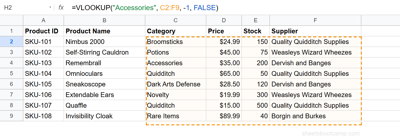
=VLOOKUP("Accessories", C2:F9, -1, FALSE)This formula breaks. There is no column “-1” in a VLOOKUP range. The column index must be a positive number, so VLOOKUP cannot reach columns to the left of the search column.
If your search column is C and you need a value from column B, VLOOKUP requires you to rearrange your data so column B comes after column C. That is not practical for shared spreadsheets with established layouts.
How INDEX MATCH Solves Left Lookups
INDEX MATCH uses two separate ranges: one for searching and one for returning. These ranges are independent, so column order does not matter.
=INDEX(return_range, MATCH(search_key, lookup_range, 0))- INDEX range — the column you want a value from (can be left, right, or anywhere)
- MATCH range — the column you are searching in
Because the two ranges are set independently, you can search column C and return from column A, column B, or any other column. The relative position does not matter.
Left Lookup: Step-by-Step
We’ll search the Category column (C) and return the Product Name (B) from the product inventory.
Sample Data
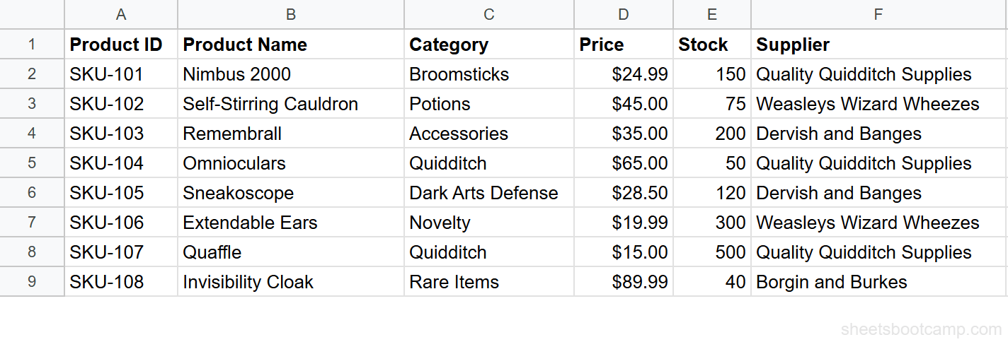
The inventory has Product ID (A), Product Name (B), Category (C), Price (D), Stock (E), and Supplier (F) with 8 products in rows 2 through 9.
Identify the left lookup scenario
You want to find the Product Name for a specific Category. Product Name is in column B (to the left) and Category is in column C (to the right). VLOOKUP would need to search C and return from B, which it cannot do.
Set the INDEX range to the left column
The return column is Product Name: B2:B9. This is the column INDEX pulls a value from.
Set the MATCH range to the right column
The search column is Category: C2:C9. MATCH looks for the search value here and returns a position number.
Combine into one formula
=INDEX(B2:B9, MATCH("Accessories", C2:C9, 0))MATCH finds “Accessories” at position 3 in C2:C9 (cell C4). INDEX returns the 3rd value from B2:B9, which is Remembrall.
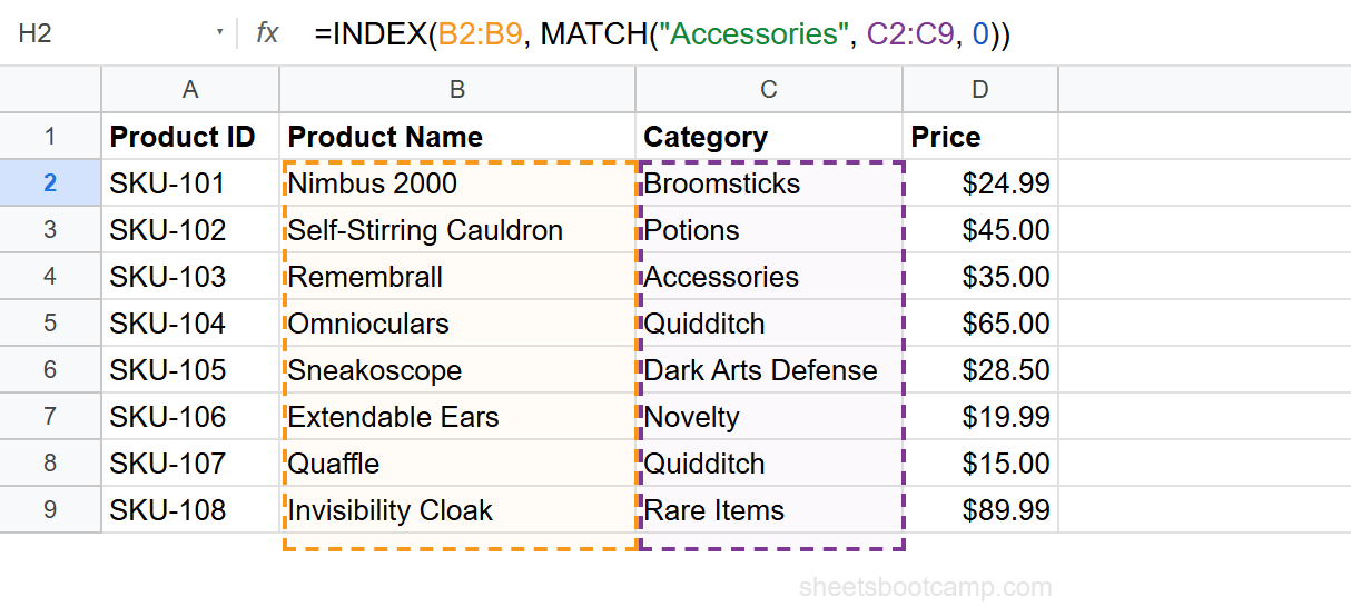
Column B is to the left of column C. INDEX MATCH does not care about column order. It treats each range as a standalone reference.
Practical Examples
Example 1: Find Product ID from Product Name
Search the Product Name column (B) and return the Product ID (A):
=INDEX(A2:A9, MATCH("Sneakoscope", B2:B9, 0))This returns SKU-105. MATCH finds “Sneakoscope” at position 5 in B2:B9, and INDEX returns the 5th value from A2:A9.
Example 2: Find Supplier from Price
Search the Price column (D) and return the Supplier (F). This is a right lookup, not a left lookup, but the formula pattern is identical:
=INDEX(F2:F9, MATCH("$89.99", D2:D9, 0))This returns Borgin and Burkes. The same formula pattern works regardless of whether the return column is left or right of the search column.
Example 3: Dynamic Left Lookup with Cell Reference
Replace the hardcoded search key with a cell reference for a reusable formula:
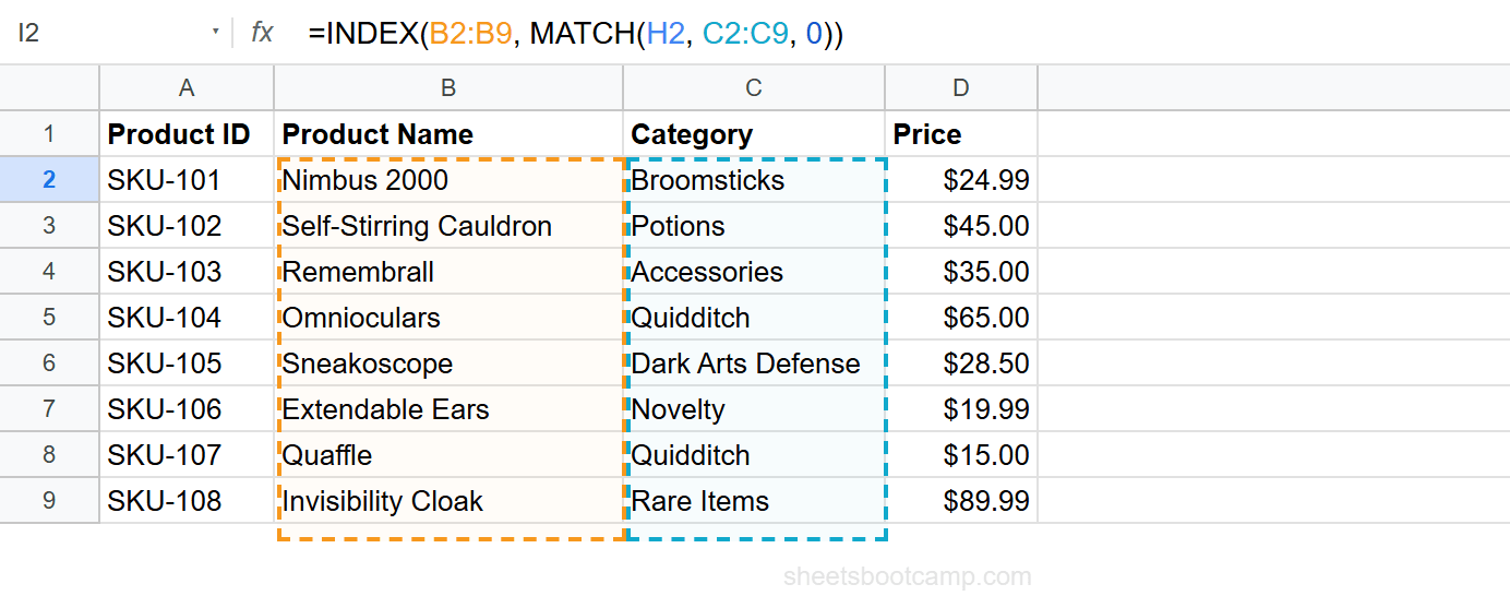
=INDEX(B2:B9, MATCH(H2, C2:C9, 0))Type any Category in cell H2. Enter “Quidditch” and the formula returns Omnioculars (the first Quidditch product). Change H2 to “Potions” and the result updates to Self-Stirring Cauldron.
If multiple rows match the search value, MATCH returns the first match only. The product inventory has two Quidditch products (Omnioculars and Quaffle). The formula returns Omnioculars because it appears first in the range. To match on additional criteria, see INDEX MATCH with multiple criteria.
XLOOKUP Alternative
XLOOKUP also handles left lookups in a single function:
=XLOOKUP("Accessories", C2:C9, B2:B9)This returns Remembrall, the same result as the INDEX MATCH version. XLOOKUP separates the search range and return range, so column order does not matter.
| Feature | INDEX MATCH | XLOOKUP |
|---|---|---|
| Left lookups | Yes | Yes |
| Formula length | Longer (two functions) | Shorter (one function) |
| Multiple criteria | Yes (array multiplication) | Requires workaround |
| Two-way lookups | Yes (dual MATCH) | Not supported natively |
| Default match type | Must specify 0 | Exact match by default |
For a standard left lookup, XLOOKUP is shorter. For multi-criteria or two-way lookups, INDEX MATCH is the better choice.
Tips
-
The formula pattern is always the same. Whether the return column is left, right, or on a different sheet, the INDEX MATCH structure does not change. Set INDEX to the return column and MATCH to the search column.
-
Lock ranges when copying down. Use
=INDEX($B$2:$B$9, MATCH(H2, $C$2:$C$9, 0))to keep the lookup and return ranges fixed while the search key shifts per row. -
Wrap in IFERROR for missing values.
=IFERROR(INDEX(B2:B9, MATCH(H2, C2:C9, 0)), "Not found")returns “Not found” instead of #N/A when the search value does not exist. -
You do not need to rearrange your data. The whole point of INDEX MATCH for left lookups is that the data stays where it is. Never restructure a shared table for a lookup formula.
Related Google Sheets Tutorials
- INDEX MATCH: The Complete Guide — Full syntax, examples, and advanced patterns
- INDEX MATCH for Beginners — Step-by-step tutorial for your first formula
- INDEX MATCH vs VLOOKUP — When to use each lookup function
- INDEX MATCH with Multiple Criteria — Match on two or more conditions
- XLOOKUP in Google Sheets — The modern alternative for left lookups
Frequently Asked Questions
Can VLOOKUP look left in Google Sheets?
No. VLOOKUP only searches the leftmost column of a range and returns values from columns to the right. If you need to return values from a column to the left of your search column, use INDEX MATCH or XLOOKUP instead.
What is a left lookup in Google Sheets?
A left lookup returns a value from a column that sits to the left of the column you are searching. For example, searching column C and returning a value from column A. INDEX MATCH handles this by letting you set each range independently.
Is INDEX MATCH the only way to do a left lookup?
No. XLOOKUP also supports left lookups in a single function. INDEX MATCH and XLOOKUP both work. Choose INDEX MATCH if you also need multiple criteria or two-way lookups.
Does the column order matter for INDEX MATCH?
No. INDEX MATCH references the lookup column and return column as separate ranges. The columns can be in any order, any distance apart, and even on different sheets.
How do I do a reverse VLOOKUP in Google Sheets?
Use INDEX MATCH. Set the INDEX range to the column you want to return from and the MATCH range to the column you want to search. The formula is =INDEX(return_range, MATCH(search_key, lookup_range, 0)).