Two-Way Lookup with INDEX MATCH in Google Sheets
Use INDEX MATCH MATCH for two-way lookups in Google Sheets. Find values at the intersection of a row and column with step-by-step examples.
Sheets Bootcamp
May 8, 2026
A two-way lookup in Google Sheets finds a value at the intersection of a specific row and column. Standard INDEX MATCH searches one column for a row position. Adding a second MATCH for the column position creates a two-dimensional lookup that works with cross-reference tables, schedules, and matrix-style data.
In This Guide
- What Is a Two-Way Lookup?
- The INDEX MATCH MATCH Pattern
- Two-Way Lookup: Step-by-Step
- Practical Examples
- Dynamic Two-Way Lookup
- Common Errors
- Tips
- Related Google Sheets Tutorials
- Frequently Asked Questions
What Is a Two-Way Lookup?
A two-way lookup answers the question: “What value sits at this row and this column?” You provide two search keys: one to identify the row and one to identify the column.
This comes up with cross-reference tables where row labels and column headers both matter. A quarterly sales report has salesperson names down the side and quarter labels across the top. To find Hermione’s Q3 sales, you need to match both the row (Hermione) and the column (Q3).
Neither VLOOKUP nor standard INDEX MATCH can handle this in a single formula. VLOOKUP hardcodes the column index as a number. Standard INDEX MATCH finds the row but returns from a fixed column. INDEX MATCH MATCH solves both at once.
The INDEX MATCH MATCH Pattern
The formula uses INDEX with three arguments: a data range, a row number from the first MATCH, and a column number from the second MATCH.
=INDEX(data_range, MATCH(row_key, row_labels, 0), MATCH(col_key, col_headers, 0))| Component | Purpose |
|---|---|
| data_range | The body of the table (no headers, no row labels) |
| MATCH(row_key, row_labels, 0) | Finds the row position of the row search key |
| MATCH(col_key, col_headers, 0) | Finds the column position of the column search key |
The first MATCH searches vertically (down a column). The second MATCH searches horizontally (across a row). INDEX returns the cell at their intersection.
Two-Way Lookup: Step-by-Step
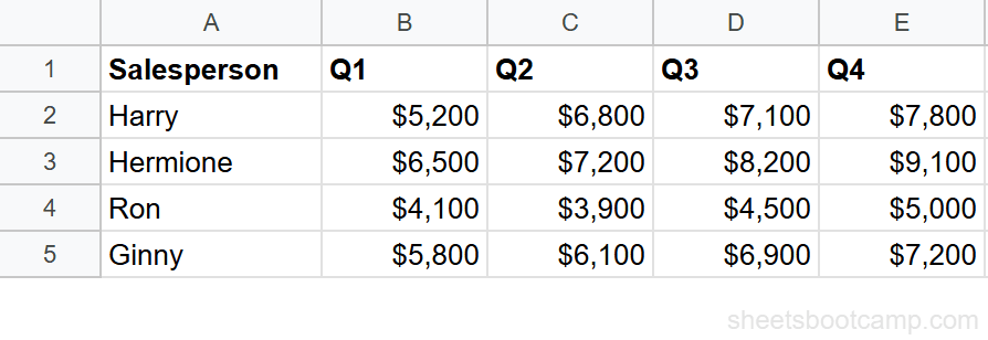
We’ll use a quarterly sales table to find a specific salesperson’s sales for a specific quarter.
Sample Data
The table has salesperson names in column A and quarterly totals in columns B through E (Q1 through Q4), with data in rows 2 through 5.
Set up your cross-reference table
The table body (B2:E5) contains the sales values. Row labels (A2:A5) contain the salesperson names. Column headers (B1:E1) contain the quarter labels Q1 through Q4.
Write the row MATCH
Find Hermione’s row position in the name column:
=MATCH("Hermione", A2:A5, 0)This returns 2 because Hermione is the 2nd value in A2:A5.
Write the column MATCH
Find Q3’s column position in the header row:
=MATCH("Q3", B1:E1, 0)This returns 3 because Q3 is the 3rd value in B1:E1.
Combine into INDEX MATCH MATCH
=INDEX(B2:E5, MATCH("Hermione", A2:A5, 0), MATCH("Q3", B1:E1, 0))- First MATCH returns 2 (Hermione’s row in the data range)
- Second MATCH returns 3 (Q3’s column in the data range)
- INDEX returns the value at row 2, column 3 of B2:E5, which is $8,200
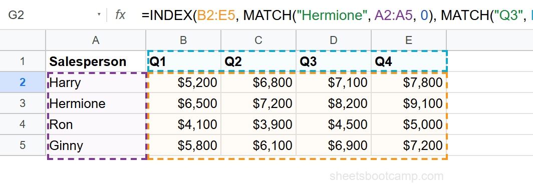
The INDEX data range must exclude the row labels and column headers. Use B2:E5 (the data body), not A1:E5. If you include the headers, the MATCH positions will point to wrong cells.
Practical Examples
Example 1: Find Ron’s Q1 Sales
=INDEX(B2:E5, MATCH("Ron", A2:A5, 0), MATCH("Q1", B1:E1, 0))MATCH finds Ron at position 3 in A2:A5, Q1 at position 1 in B1:E1. INDEX returns $4,100 from row 3, column 1 of the data range.
Example 2: Find Harry’s Q4 Sales
=INDEX(B2:E5, MATCH("Harry", A2:A5, 0), MATCH("Q4", B1:E1, 0))MATCH finds Harry at position 1, Q4 at position 4. INDEX returns $7,800 from row 1, column 4.
Example 3: Use with Product Inventory Data
The pattern works with any cross-reference layout. Using the product inventory, if you had a matrix of products by attribute, the formula structure stays the same.
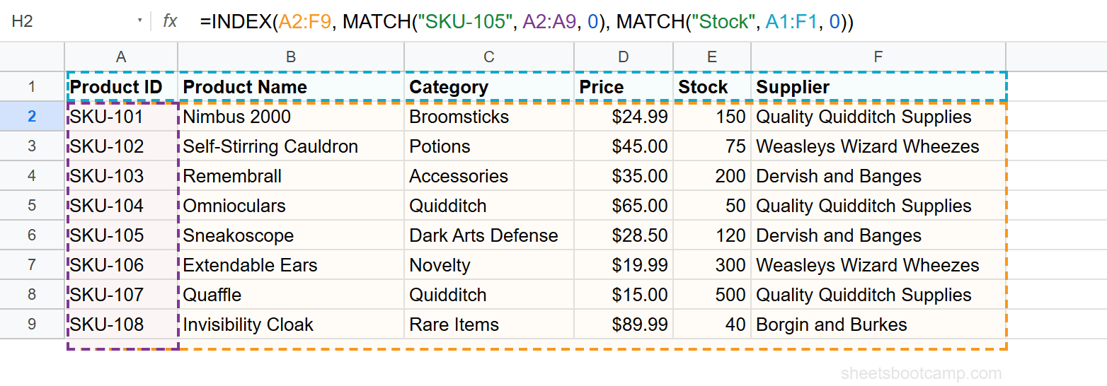
To find a specific product’s stock from the standard inventory table, you could also write a two-way lookup with INDEX over a multi-column range:
=INDEX(A2:F9, MATCH("SKU-105", A2:A9, 0), MATCH("Stock", A1:F1, 0))This returns 120 — the stock count for SKU-105 (Sneakoscope). The first MATCH finds SKU-105 at row position 5, the second MATCH finds “Stock” at column position 5 in the headers.
Dynamic Two-Way Lookup
Replace hardcoded values with cell references to create a reusable lookup:
=INDEX(B2:E5, MATCH(G2, A2:A5, 0), MATCH(H2, B1:E1, 0))Type a salesperson name in G2 and a quarter label in H2. The formula returns the matching sales figure. Pair this with data validation dropdowns to build an interactive dashboard.
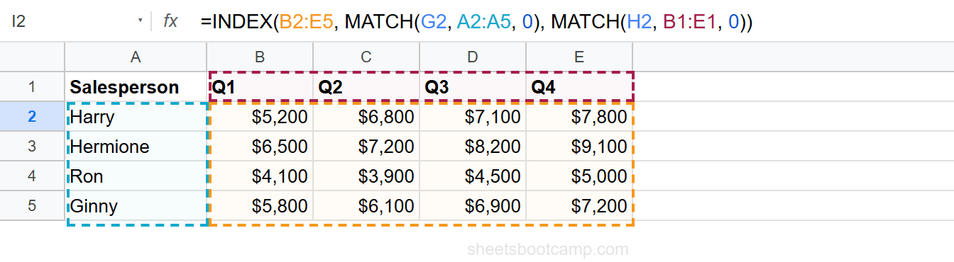
Lock the ranges with absolute references when copying the formula: =INDEX($B$2:$E$5, MATCH(G2, $A$2:$A$5, 0), MATCH(H2, $B$1:$E$1, 0)). The cell references G2 and H2 stay relative.
Common Errors
#N/A — Search key not found
One or both MATCH functions cannot find the search key. Check spelling, extra spaces, and data types. “Q 3” (with a space) does not match “Q3”.
Fix: Verify the row label and column header exist exactly as typed. Use =TRIM() to remove whitespace.
#REF! — Data range too small
The MATCH position exceeds the dimensions of the INDEX range. If MATCH returns row position 5 but the INDEX range has only 4 rows, you get #REF!.
Fix: Make sure the INDEX data range covers all rows and columns. If the table has 4 salesperson rows (2 through 5), the data range should be B2:E5.
Wrong value — Headers included in data range
If the INDEX range includes the header row (B1:E5 instead of B2:E5), positions shift by one row. MATCH returns position 2 for Hermione, but row 2 of B1:E5 is actually Harry’s data.
Fix: Start the INDEX range at the first data row, not the header row.
Both MATCH functions must use 0 for exact matching. The default (1) assumes sorted data and returns approximate matches, which produces wrong positions on unsorted row labels or column headers.
Tips
-
Keep the data range clean. The INDEX range should cover only the table body. Row labels and column headers go in the MATCH ranges, not the INDEX range.
-
Test each MATCH separately. Before writing the full formula, test
=MATCH("Hermione", A2:A5, 0)and=MATCH("Q3", B1:E1, 0)individually. Confirm both return the expected positions. -
Use IFERROR for missing combinations.
=IFERROR(INDEX(..., MATCH(...), MATCH(...)), "Not found")handles cases where the row or column key does not exist. -
This pattern is unique to INDEX MATCH. Neither VLOOKUP nor XLOOKUP supports true two-way lookups natively. INDEX MATCH MATCH is the standard approach for matrix-style data.
Related Google Sheets Tutorials
- INDEX MATCH: The Complete Guide — Full syntax, left lookups, and the combined formula pattern
- INDEX MATCH for Beginners — Start here if you are new to INDEX MATCH
- INDEX MATCH with Multiple Criteria — Match on two or more conditions using array multiplication
- INDEX MATCH vs VLOOKUP — When to use each lookup function
- VLOOKUP: The Complete Guide — Full VLOOKUP reference with examples
Frequently Asked Questions
What is a two-way lookup in Google Sheets?
A two-way lookup finds a value at the intersection of a specific row and column. You provide both a row identifier and a column header, and the formula returns the cell where they meet. INDEX with two MATCH functions handles this.
Can VLOOKUP do a two-way lookup?
VLOOKUP alone cannot do a two-way lookup. You can nest MATCH inside the column index argument of VLOOKUP, but INDEX MATCH MATCH is the standard approach and easier to read.
What does INDEX MATCH MATCH mean?
INDEX MATCH MATCH is a formula pattern that uses INDEX with two MATCH functions. The first MATCH finds the row position, the second MATCH finds the column position, and INDEX returns the value at that intersection.
Why does my two-way lookup return the wrong value?
Check that both MATCH functions use 0 for exact matching. Also verify the row headers and column headers in your data match the search values exactly, including spelling and spacing.
Can XLOOKUP do a two-way lookup?
XLOOKUP does not support two-way lookups natively. You can nest two XLOOKUP functions, but INDEX MATCH MATCH is more readable and widely used for this purpose.