INDEX MATCH vs VLOOKUP in Google Sheets
Compare INDEX MATCH and VLOOKUP in Google Sheets. See when each lookup formula works best with side-by-side examples, performance notes, and migration tips.
Sheets Bootcamp
March 13, 2026
INDEX MATCH and VLOOKUP both look up values in a table, but they work differently under the hood. VLOOKUP packs everything into one function. INDEX MATCH splits the job between two functions, which gives it more flexibility at the cost of a longer formula.
This guide compares both approaches side by side, shows where each one works best, and explains how to convert VLOOKUP formulas to INDEX MATCH when needed.
In This Guide
- The Same Lookup, Two Ways
- Key Differences
- When VLOOKUP Wins
- When INDEX MATCH Wins
- Column Insertion: The Silent Problem
- How to Convert VLOOKUP to INDEX MATCH
- What About XLOOKUP?
- Related Google Sheets Tutorials
- Frequently Asked Questions
The Same Lookup, Two Ways
Both formulas answer the same question: “What is the price for SKU-103?” using the product inventory table.
VLOOKUP approach:
=VLOOKUP("SKU-103", A2:D9, 4, FALSE)This searches for SKU-103 in the first column of A2:D9 and returns the value from column 4 (Price). Result: $35.00.
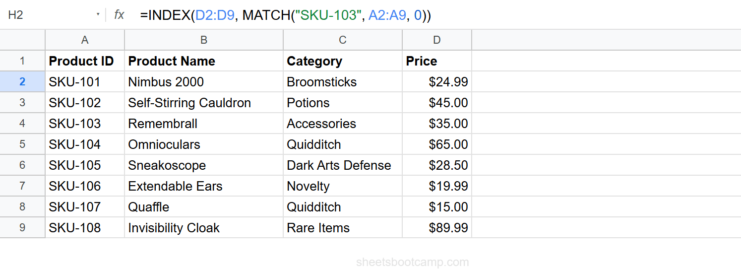
INDEX MATCH approach:
=INDEX(D2:D9, MATCH("SKU-103", A2:A9, 0))MATCH finds SKU-103 at position 3 in A2:A9. INDEX returns the 3rd value from D2:D9. Result: $35.00.
Same answer, different paths. The question is which path works better for your situation.
Key Differences
| Feature | VLOOKUP | INDEX MATCH |
|---|---|---|
| Lookup direction | Right only (leftmost column) | Any direction |
| Column insertions | Breaks silently (index shifts) | Safe (references specific ranges) |
| Formula length | Shorter (one function) | Longer (two functions) |
| Readability | Easier to scan | Takes practice to read |
| Multiple criteria | Requires helper column | Built-in with array multiplication |
| Two-way lookups | Not possible | Supported with dual MATCH |
| Return column | Uses a number (e.g., 4) | References the range directly (D2:D9) |
The most important differences are lookup direction and column-insertion safety. Everything else is a tradeoff between simplicity and flexibility.
When VLOOKUP Wins
VLOOKUP is the better choice when three conditions are true:
- The search column is the leftmost column in your range. VLOOKUP requires this.
- The table structure is stable. No one is adding or removing columns between your search column and return column.
- Readability matters. VLOOKUP communicates its purpose in a single function call. In shared spreadsheets where colleagues review formulas,
=VLOOKUP("SKU-103", A2:D9, 4, FALSE)is faster to understand than the INDEX MATCH equivalent.
A standard product lookup, employee directory search, or price check — if the data layout fits, VLOOKUP is the straightforward choice.
=VLOOKUP(H2, A2:D9, 4, FALSE)One function, four arguments, done.
When INDEX MATCH Wins
INDEX MATCH is the better choice when any of these are true:
Left lookups
You want to return a value from a column to the left of your search column. VLOOKUP cannot do this.
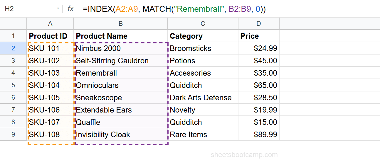
For example, finding the Product ID (column A) when you know the Product Name (column B):
=INDEX(A2:A9, MATCH("Remembrall", B2:B9, 0))This returns SKU-103 by searching column B and returning from column A. VLOOKUP would require rearranging your data to put Product Name in the leftmost column.
Column-insertion safety
Your table structure changes over time. Team members add new columns, rearrange data, or import columns from other sheets. INDEX MATCH references each range directly, so these changes do not affect the formula.
Multiple criteria
You need to match on two or more conditions. INDEX MATCH handles this natively with array multiplication:
=INDEX(D2:D9, MATCH(1, (A2:A9="SKU-107")*(C2:C9="Quidditch"), 0))VLOOKUP would require a helper column that concatenates the criteria before searching.
Shared spreadsheets with frequent edits
When multiple people work in the same spreadsheet and regularly add or move columns, VLOOKUP formulas break without warning. INDEX MATCH is the safer option for collaborative spreadsheets.
If you are building a spreadsheet for yourself and the layout is fixed, VLOOKUP is fine. If other people will edit the structure, INDEX MATCH is the lower-risk choice.
Column Insertion: The Silent Problem
This is the most important practical difference between the two formulas.
Starting point: You have a VLOOKUP formula that returns the price (column D, the 4th column in the range):
=VLOOKUP("SKU-103", A2:D9, 4, FALSE)This works. The price for SKU-103 is $35.00.
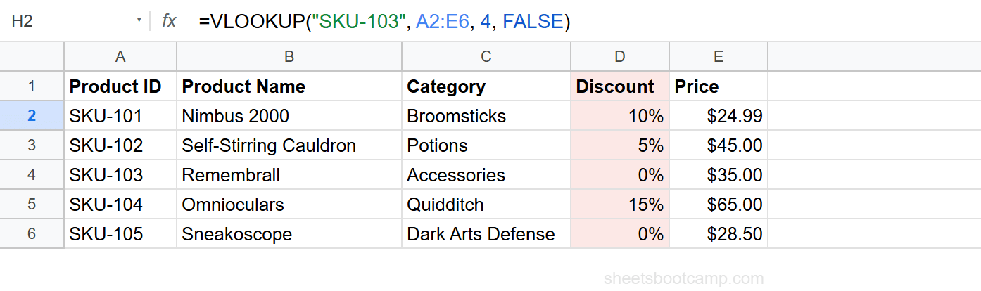
What happens when a column is inserted: Someone adds a “Discount” column between Category (C) and Price (D). Price moves from column D to column E, becoming the 5th column in the range.
The VLOOKUP formula still says 4. It now returns the Discount column instead of Price. No error appears. The formula returns a wrong value silently.
INDEX MATCH handles this automatically:
=INDEX(D2:D9, MATCH("SKU-103", A2:A9, 0))When the new column is inserted, Google Sheets updates the INDEX range from D2:D9 to E2:E9. The formula continues to return the correct price. No manual update needed.
VLOOKUP’s column index is a hardcoded number. It does not update when columns move. INDEX MATCH uses range references that Google Sheets adjusts automatically during column insertions and deletions.
How to Convert VLOOKUP to INDEX MATCH
The conversion follows a consistent pattern. Take any VLOOKUP formula:
=VLOOKUP(search_key, range, column_index, FALSE)Rewrite it as:
=INDEX(return_column_range, MATCH(search_key, lookup_column_range, 0))Conversion example
Original VLOOKUP:
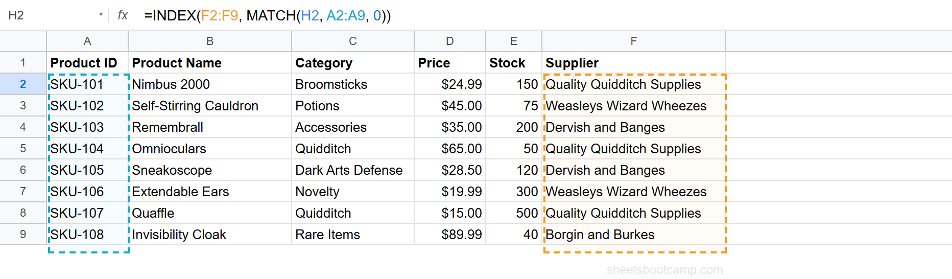
=VLOOKUP(H2, A2:F9, 6, FALSE)This searches H2 in the first column (A) of A2:F9 and returns column 6 (Supplier, column F).
Converted to INDEX MATCH:
=INDEX(F2:F9, MATCH(H2, A2:A9, 0))F2:F9replaces column index6— this is the Supplier column directlyA2:A9is the first column of the original range (where VLOOKUP searched)H2stays the same (the search key)0replacesFALSE(exact match)
Step-by-step conversion
- Identify the search key — the first argument in VLOOKUP. It stays the same.
- Identify the lookup column — the first column of the VLOOKUP range. This becomes the MATCH range.
- Identify the return column — count the column_index from the VLOOKUP range. That column becomes the INDEX range.
- Replace FALSE with 0 — both mean exact match, but MATCH uses
0instead ofFALSE.
You do not need to convert working VLOOKUP formulas unless you have a specific reason. If the formula returns the correct result and your table structure is stable, leave it as is.
What About XLOOKUP?
Google Sheets added XLOOKUP to address VLOOKUP’s limitations. XLOOKUP handles left lookups, defaults to exact match, and uses a single function.
=XLOOKUP("SKU-103", A2:A9, D2:D9)This is shorter than INDEX MATCH and avoids the column index problem from VLOOKUP. For many use cases, XLOOKUP is the modern replacement for both.
However, INDEX MATCH still has two advantages over XLOOKUP:
- Two-way lookups — INDEX with two MATCH functions can find a value at the intersection of a row and column. XLOOKUP does not support this natively.
- Array-based multiple criteria — the
MATCH(1, (condition1)*(condition2), 0)pattern is not available in XLOOKUP without workarounds.
If you need standard lookups in any direction, XLOOKUP is the simplest choice. If you need two-way lookups or multi-criteria matching, INDEX MATCH remains the go-to option.
Related Google Sheets Tutorials
- INDEX MATCH: The Complete Guide — Full syntax, examples, and advanced patterns
- INDEX MATCH for Beginners — Step-by-step tutorial for your first INDEX MATCH formula
- INDEX MATCH with Multiple Criteria — Match on two or more conditions
- VLOOKUP: The Complete Guide — VLOOKUP syntax, examples, and error fixes
- Fix VLOOKUP Errors — Troubleshoot #N/A, #REF!, and #VALUE! in VLOOKUP
Frequently Asked Questions
Is INDEX MATCH faster than VLOOKUP in Google Sheets?
For single lookups, the difference is negligible. For large datasets with thousands of rows, INDEX MATCH can be marginally faster because MATCH searches a single column rather than scanning a multi-column range. In practice, both perform well for most spreadsheets.
Should I always use INDEX MATCH instead of VLOOKUP?
No. VLOOKUP is easier to read and write for standard lookups where the search column is leftmost and the table structure is stable. Use INDEX MATCH when you need left lookups, column-insertion safety, or multiple criteria.
Can I replace all my VLOOKUP formulas with INDEX MATCH?
Yes. Every VLOOKUP formula can be rewritten as INDEX MATCH. Replace =VLOOKUP(key, range, col, FALSE) with =INDEX(return_column, MATCH(key, lookup_column, 0)). Whether you should depends on whether the added flexibility justifies the longer formula.
Does INDEX MATCH work the same in Google Sheets and Excel?
The syntax is identical. Both platforms support INDEX, MATCH, and their combination. The behavior and results are the same.
What about XLOOKUP vs INDEX MATCH?
XLOOKUP was designed to replace both VLOOKUP and INDEX MATCH with a single function. It handles left lookups and defaults to exact match. However, INDEX MATCH still offers two-way lookups and array-based multiple criteria matching that XLOOKUP does not support natively.