Named Ranges in Google Sheets: Create and Use Them
Learn how to create and use named ranges in Google Sheets. Replace cell references with readable names in formulas. Covers creation, editing, and best practices.
Sheets Bootcamp
June 23, 2026
Named ranges in Google Sheets let you assign a descriptive name to a cell or range of cells, then use that name in formulas instead of cell references. =SUM(Revenue) is easier to read and maintain than =SUM(Sheet2!B2:B13).
This guide covers how to create, edit, and manage named ranges, plus practical examples of using them in formulas, data validation, and the INDIRECT function.
In This Guide
- What Are Named Ranges?
- Syntax and Parameters
- How to Create Named Ranges: Step-by-Step
- Named Range Examples
- Common Errors and How to Fix Them
- Tips and Best Practices
- Related Google Sheets Tutorials
- FAQ
What Are Named Ranges?
A named range is an alias for a cell address. Instead of writing =VLOOKUP(A2, Sheet2!A:D, 3, FALSE), you define the range Sheet2!A:D as “ProductTable” and write =VLOOKUP(A2, ProductTable, 3, FALSE).
Named ranges make formulas self-documenting. When you open a spreadsheet months later, =SUMIF(Department, "Sales", Salary) tells you exactly what the formula calculates. =SUMIF(C2:C50, "Sales", F2:F50) requires you to check what’s in columns C and F.
Syntax and Parameters
Named ranges aren’t a function — they’re a feature you use inside functions. Here’s how they work in formulas:
=SUM(Revenue)| Element | Description |
|---|---|
| Revenue | A named range pointing to cells B2:B13. Used anywhere a cell reference would go |
Naming Rules
| Rule | Example | Invalid |
|---|---|---|
| Must start with a letter or underscore | Revenue, _temp | 2024Revenue |
| Letters, numbers, underscores, periods only | Q1_Revenue, data.2024 | Q1 Revenue |
| No spaces | Total_Sales | Total Sales |
| Case-insensitive | Revenue = revenue = REVENUE | — |
| Can’t be a cell reference | Sales (valid) | A1 (conflicts with cell A1) |
Don’t name a range something that looks like a cell reference. Names like “B2” or “R1C1” conflict with the cell reference system and cause errors.
How to Create Named Ranges: Step-by-Step
We’ll name a range of monthly revenue data and use it in a SUM formula.
Select the range to name
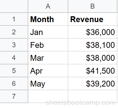
Highlight cells B2:B13, which contain 12 months of revenue values.

Create the named range
Go to Data > Named ranges. The sidebar opens with your selected range pre-filled. Type “Revenue” as the name and click Done.
Shortcut: Select your range, click the Name Box (the small box to the left of the formula bar that shows the cell address), type the name, and press Enter. This is faster than using the Data menu.
Use the named range in a formula
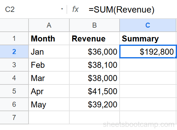
In any cell, type the formula using the name instead of the cell reference:
=SUM(Revenue)Google Sheets recognizes “Revenue” and calculates the sum of B2:B13. As you type, Sheets auto-suggests matching named ranges.
Named Range Examples
Use in VLOOKUP
Name the range A1:D50 as “Products” and use it as the VLOOKUP table array:
=VLOOKUP("SKU-102", Products, 3, FALSE)This is clearer than =VLOOKUP("SKU-102", Sheet2!A1:D50, 3, FALSE) and doesn’t require the reader to know what lives on Sheet2 in columns A through D.
Use in SUMIF
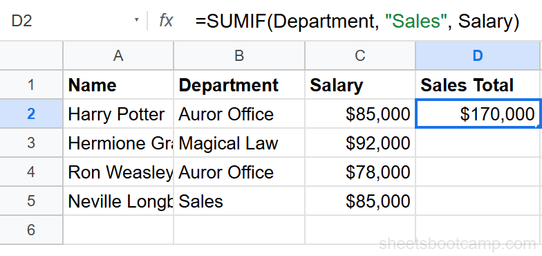
Name C2:C50 as “Department” and F2:F50 as “Salary” to write readable conditional sums:
=SUMIF(Department, "Sales", Salary)Anyone reading this formula understands it sums the Salary column where the Department column equals “Sales.”
Use with INDIRECT for Dynamic References
Combine named ranges with INDIRECT to reference different ranges based on a cell value. If you have named ranges “Sales_Q1”, “Sales_Q2”, “Sales_Q3”, and “Sales_Q4”:
=SUM(INDIRECT("Sales_"&A1))When A1 contains “Q2”, this evaluates to =SUM(Sales_Q2). Change A1 to “Q3” and the formula sums a different named range.
Common Errors and How to Fix Them
#NAME? Error
The named range doesn’t exist or is misspelled. Open Data > Named ranges and verify the exact name. Names are case-insensitive, but typos like “Revenu” instead of “Revenue” cause this error.
#REF! Error
The named range was deleted or the underlying cells were removed. If you delete rows that a named range points to, the range breaks. Recreate the named range pointing to the correct cells.
Formula Shows the Name as Text
You typed the name inside quotes: =SUM("Revenue"). Remove the quotes. Named ranges are used without quotes in formulas: =SUM(Revenue).
Start typing a named range in a formula and Google Sheets shows an autocomplete dropdown. Select from the list to avoid typos.
Tips and Best Practices
-
Use descriptive, consistent names.
MonthlyRevenueis better thandata1. Adopt a naming convention like Category_Metric (e.g., Sales_Revenue, HR_Salary) and stick with it. -
Named ranges work across sheets. A range named “Products” on Sheet1 can be used on any tab without a sheet prefix. This makes cross-sheet formulas cleaner.
-
Audit your named ranges regularly. Go to Data > Named ranges to see all names and their targets. Delete unused ranges to avoid confusion. Names pointing to deleted cells show #REF! in the sidebar.
-
Use named ranges in data validation. Set a dropdown source to a named range instead of a cell reference. If the source data moves, update the named range once rather than every validation rule.
-
Named ranges make shared spreadsheets easier to maintain. Other people using your sheet can read
=VLOOKUP(A2, Products, 3, FALSE)and understand it without tracking down which cells “Products” refers to.
Related Google Sheets Tutorials
- INDIRECT Function in Google Sheets - Build dynamic references to named ranges using INDIRECT
- Absolute vs Relative References - Understand the cell reference system that named ranges simplify
- Drop-Down List in Google Sheets - Use named ranges as dropdown sources for cleaner validation rules
- VLOOKUP: The Complete Guide - Replace VLOOKUP range references with named ranges for readable formulas
FAQ
How do I create a named range in Google Sheets?
Select the cells, go to Data > Named ranges, type a name, and click Done. You can also select the range, click the Name Box (left of the formula bar), type the name, and press Enter. Names must start with a letter and can’t contain spaces.
How do I use a named range in a formula?
Type the name directly in your formula: =SUM(Revenue) instead of =SUM(B2:B13). Google Sheets auto-suggests named ranges as you type. Named ranges work in any function — VLOOKUP, IF, SUMIF, QUERY, and more.
Can I use named ranges across sheets?
Yes. Named ranges are scoped to the entire spreadsheet, not a single sheet. A range named Revenue on Sheet1 can be used in formulas on Sheet2 without any sheet prefix. Type =SUM(Revenue) on any tab and it resolves correctly.
How do I edit or delete a named range?
Go to Data > Named ranges to open the sidebar. Find the name, click the pencil icon to edit the range or name, or click the trash icon to delete it. Deleting a named range breaks any formulas that reference it.
What are the naming rules for named ranges?
Names must start with a letter or underscore. They can contain letters, numbers, underscores, and periods. Spaces are not allowed — use underscores instead (e.g., Q1_Revenue). Names are case-insensitive, so Revenue and revenue refer to the same range.
Can I use named ranges in data validation?
Yes. When creating a dropdown list from a range, type the named range in the criteria field. For example, set the data validation source to =ProductList instead of Sheet2!A2:A50. This keeps the validation rule readable and easier to maintain.