QUERY with IMPORTRANGE in Google Sheets
Learn how to combine QUERY with IMPORTRANGE in Google Sheets to filter, sort, and summarize data from another spreadsheet. Step-by-step examples.
Sheets Bootcamp
May 6, 2026
QUERY with IMPORTRANGE in Google Sheets lets you pull data from another spreadsheet and filter, sort, or summarize it in a single formula. Instead of importing an entire sheet and then writing a separate QUERY on the local copy, you wrap IMPORTRANGE inside QUERY to do both in one step. We’ll cover the syntax, the access permission step, and how to filter and aggregate imported data.
In This Guide
- Syntax
- How to Use QUERY with IMPORTRANGE: Step-by-Step
- Filter Imported Data with WHERE
- Sort and Limit Imported Data
- Aggregate Imported Data with GROUP BY
- Combine Local and Imported Data
- Common Errors
- Tips
- Related Google Sheets Tutorials
- FAQ
Syntax
QUERY wraps IMPORTRANGE as its data source:
=QUERY(IMPORTRANGE("spreadsheet_url", "range"), "query_string")| Part | Role | Example |
|---|---|---|
spreadsheet_url | Full URL of the external spreadsheet | "https://docs.google.com/spreadsheets/d/abc123/edit" |
range | Sheet name and cell range | "Sheet1!A1:G" |
query_string | Standard QUERY syntax with Col notation | "SELECT Col2, Col6 WHERE Col3 = 'Hogwarts'" |
IMPORTRANGE returns an array, so you must use Col1, Col2, Col3 notation in the query string — not A, B, C. This is the same rule as QUERY with combined ranges.
How to Use QUERY with IMPORTRANGE: Step-by-Step
This example queries sales records stored in a separate spreadsheet.
Grant access to the external spreadsheet
Before combining QUERY and IMPORTRANGE, you need to authorize access. In an empty cell, enter IMPORTRANGE alone:
=IMPORTRANGE("https://docs.google.com/spreadsheets/d/abc123/edit", "Sheet1!A1:G11")Google Sheets displays an “Allow access” prompt. Click it to grant permission. This is a one-time step per external spreadsheet. See IMPORTRANGE Access Permission for troubleshooting.
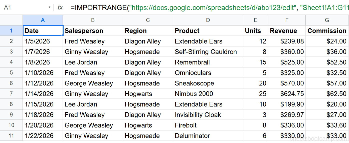
Verify the imported data
After granting access, the cell displays the external data. Confirm the columns are correct: Date (Col1), Salesperson (Col2), Region (Col3), Product (Col4), Units (Col5), Revenue (Col6), Commission (Col7).
Wrap in QUERY to filter and sort
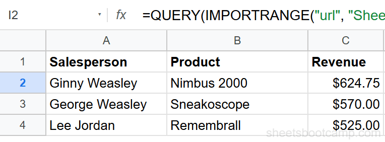
Replace the formula with:
=QUERY(IMPORTRANGE("https://docs.google.com/spreadsheets/d/abc123/edit", "Sheet1!A1:G11"), "SELECT Col2, Col4, Col6 WHERE Col6 > 400 ORDER BY Col6 DESC")This imports the 10-row dataset and returns Salesperson, Product, and Revenue for transactions over $400, sorted by revenue descending. Three rows match: Ginny Weasley’s Nimbus 2000 ($624.75), George Weasley’s Sneakoscope ($570.00), and Lee Jordan’s Remembrall ($525.00).
The access grant persists after you change the formula. You can add QUERY around IMPORTRANGE without re-authorizing. The grant applies to the entire external spreadsheet, not a specific range.
Filter Imported Data with WHERE
WHERE filters rows from the imported data:
=QUERY(IMPORTRANGE("url", "Sheet1!A1:G11"), "SELECT * WHERE Col3 = 'Hogsmeade'")This returns only rows where Region (Col3) equals Hogsmeade. Text values still need single quotes inside the query string.
For numeric filters:
=QUERY(IMPORTRANGE("url", "Sheet1!A1:G11"), "SELECT Col2, Col6 WHERE Col6 >= 300 AND Col6 <= 500")This returns Salesperson and Revenue for transactions between $300 and $500.
Sort and Limit Imported Data
ORDER BY sorts the imported results:
=QUERY(IMPORTRANGE("url", "Sheet1!A1:G11"), "SELECT Col2, Col6 ORDER BY Col6 DESC LIMIT 5")This returns the top 5 revenue transactions from the external spreadsheet, sorted from highest to lowest. LIMIT caps the output to 5 rows, which is useful when you only need a summary.
Aggregate Imported Data with GROUP BY
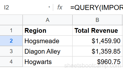
GROUP BY aggregates the imported data:
=QUERY(IMPORTRANGE("url", "Sheet1!A1:G11"), "SELECT Col3, SUM(Col6) GROUP BY Col3 ORDER BY SUM(Col6) DESC LABEL SUM(Col6) 'Total Revenue'")This imports the sales data, groups by Region (Col3), sums Revenue (Col6), and sorts by total descending. The result shows Hogsmeade ($1,459.90), Diagon Alley ($1,359.85), and Hogwarts ($960.75).
Combine Local and Imported Data
You can stack local data with imported data using curly braces, then QUERY the combined set:
=QUERY({A2:G11;IMPORTRANGE("url", "Sheet1!A2:G11")}, "SELECT * WHERE Col1 is not null")This combines your local rows (A2:G11) with imported rows into one dataset. Use Col notation for the query string. See QUERY Multiple Ranges for the full pattern.
Both ranges must have the same number of columns. If your local range has 7 columns, the imported range must also have 7 columns. Mismatched column counts cause an error.
Common Errors
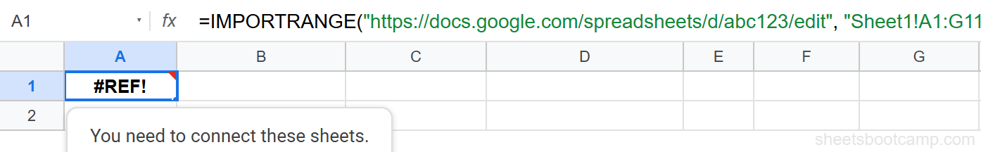
#REF! — Access not granted
The most common error. IMPORTRANGE requires a one-time access grant. Enter =IMPORTRANGE("url", "range") alone first, click “Allow access,” then build the QUERY around it.
#VALUE! — Using A, B, C instead of Col notation
SELECT A, B causes an error when IMPORTRANGE is the data source. Use SELECT Col1, Col2 instead. This is required because IMPORTRANGE returns an array without column letters.
#N/A — Wrong spreadsheet URL
Double-check the URL. It must be the full URL of the external spreadsheet, including https://. A partial URL or spreadsheet ID alone does not work.
Slow performance
IMPORTRANGE fetches data over the network on every recalculation. For large ranges, this can be slow. Narrow the range to include only the columns you need: use "Sheet1!A1:F" instead of "Sheet1!A1:Z" if you only need columns A through F. See IMPORTRANGE performance tips for more options.
Tips
1. Grant access before building the formula. Always test IMPORTRANGE alone first. Once access is granted, wrapping it in QUERY works without re-authorization.
2. Use a named range or cell for the URL. Store the spreadsheet URL in a cell (like Z1) and reference it: IMPORTRANGE(Z1, "Sheet1!A1:G"). This makes it easier to update the URL later without editing complex formulas.
3. Narrow the import range. Instead of importing entire columns (A:G), specify the data range (A1:G100). This reduces the data transferred and speeds up the formula.
For basic data imports without filtering, IMPORTRANGE alone is sufficient. Add QUERY when you need to filter, sort, or aggregate the imported data in the same formula.
Related Google Sheets Tutorials
- QUERY Function: Complete Guide — covers all QUERY clauses with syntax and examples
- QUERY WHERE Clause — filter rows with conditions
- QUERY Multiple Ranges — combine data from multiple sheets and ranges
- IMPORTRANGE Function — pull data from other spreadsheets
Frequently Asked Questions
How do you use QUERY with IMPORTRANGE in Google Sheets?
Wrap IMPORTRANGE inside QUERY: =QUERY(IMPORTRANGE("url", "Sheet1!A1:G"), "SELECT Col2, Col6 WHERE Col3 = 'Hogwarts'"). Use Col1, Col2, Col3 notation because IMPORTRANGE returns an array without column letters.
Why does QUERY with IMPORTRANGE show #REF! error?
The most common cause is that you have not granted access to the external spreadsheet. Enter the IMPORTRANGE formula alone first, click Allow access in the prompt, then build the QUERY around it. The access grant persists after you modify the formula.
Do you use A, B, C or Col1, Col2, Col3 with QUERY IMPORTRANGE?
Use Col1, Col2, Col3 notation. IMPORTRANGE returns an array without column letters, so QUERY cannot use A, B, C references. Col1 is the first column, Col2 is the second, and so on.
Can you filter IMPORTRANGE data with QUERY WHERE?
Yes. Add a WHERE clause to filter the imported data: =QUERY(IMPORTRANGE("url", "Sheet1!A1:G"), "SELECT * WHERE Col6 > 400"). This imports the data and returns only rows where column 6 exceeds 400.
Is QUERY with IMPORTRANGE slow?
IMPORTRANGE fetches data from another spreadsheet over the network, which adds latency. The QUERY itself runs fast, but the initial data fetch may take a few seconds. For large datasets, consider importing a narrower range to reduce the amount of data transferred.