QUERY Multiple Ranges in Google Sheets
Learn how to use QUERY across multiple ranges and sheets in Google Sheets. Combine data with curly braces, IMPORTRANGE, and vertical stacking.
Sheets Bootcamp
May 4, 2026
QUERY in Google Sheets can pull data from multiple ranges and sheets in a single formula. You combine ranges using curly braces ({}), then QUERY filters and sorts the combined dataset. This is useful when your data is split across tabs — monthly reports on separate sheets, regional data in different ranges, or imported data alongside local data. We’ll cover vertical stacking, column notation, and filtering across combined ranges.
In This Guide
- How Curly Braces Combine Ranges
- How to QUERY Multiple Ranges: Step-by-Step
- Col1, Col2 Notation
- Combine Ranges from Different Sheets
- Filter and Sort Combined Data
- Combine with IMPORTRANGE
- Common Mistakes
- Tips
- Related Google Sheets Tutorials
- FAQ
How Curly Braces Combine Ranges
Curly braces create arrays in Google Sheets. The separator determines how ranges combine:
| Separator | Effect | Example |
|---|---|---|
; (semicolon) | Stacks vertically (adds rows) | {A1:C5;A8:C12} |
, (comma) | Places side by side (adds columns) | {A1:B5,D1:E5} |
For QUERY across multiple ranges, vertical stacking (semicolons) is the standard pattern. All ranges must have the same number of columns.
When you combine ranges with curly braces, the result loses its column letters. You must use Col1, Col2, Col3 notation instead of A, B, C in the query string. This is the most common source of errors when querying combined ranges.
How to QUERY Multiple Ranges: Step-by-Step
We’ll use the sales records from the QUERY guide. Imagine the first 10 rows (January sales) are on one sheet and the remaining rows (February sales) are on another sheet.
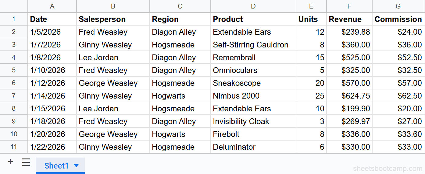
Jan Sales (Sheet1): A1:G11
| A | B | C | D | E | F | G | |
|---|---|---|---|---|---|---|---|
| 1 | Date | Salesperson | Region | Product | Units | Revenue | Commission |
| 2 | 1/5/2026 | Fred Weasley | Diagon Alley | Extendable Ears | 12 | $239.88 | $24.00 |
| 3 | 1/7/2026 | Ginny Weasley | Hogsmeade | Self-Stirring Cauldron | 8 | $360.00 | $36.00 |
| … | |||||||
| 11 | 1/22/2026 | Ginny Weasley | Hogsmeade | Deluminator | 6 | $330.00 | $33.00 |
Feb Sales (Sheet2): A1:G4
| A | B | C | D | E | F | G | |
|---|---|---|---|---|---|---|---|
| 1 | Date | Salesperson | Region | Product | Units | Revenue | Commission |
| 2 | 2/1/2026 | Lee Jordan | Hogwarts | Omnioculars | 7 | $455.00 | $45.50 |
| 3 | 2/3/2026 | Fred Weasley | Diagon Alley | Nimbus 2000 | 15 | $374.85 | $37.50 |
| 4 | 2/5/2026 | George Weasley | Hogsmeade | Extendable Ears | 14 | $279.86 | $28.00 |
Set up data on two sheets
Your January data lives on a sheet named “Jan Sales” in A1:G11 (10 data rows). February data lives on “Feb Sales” in A1:G4 (3 data rows). Both sheets have the same column structure.
Combine ranges with curly braces
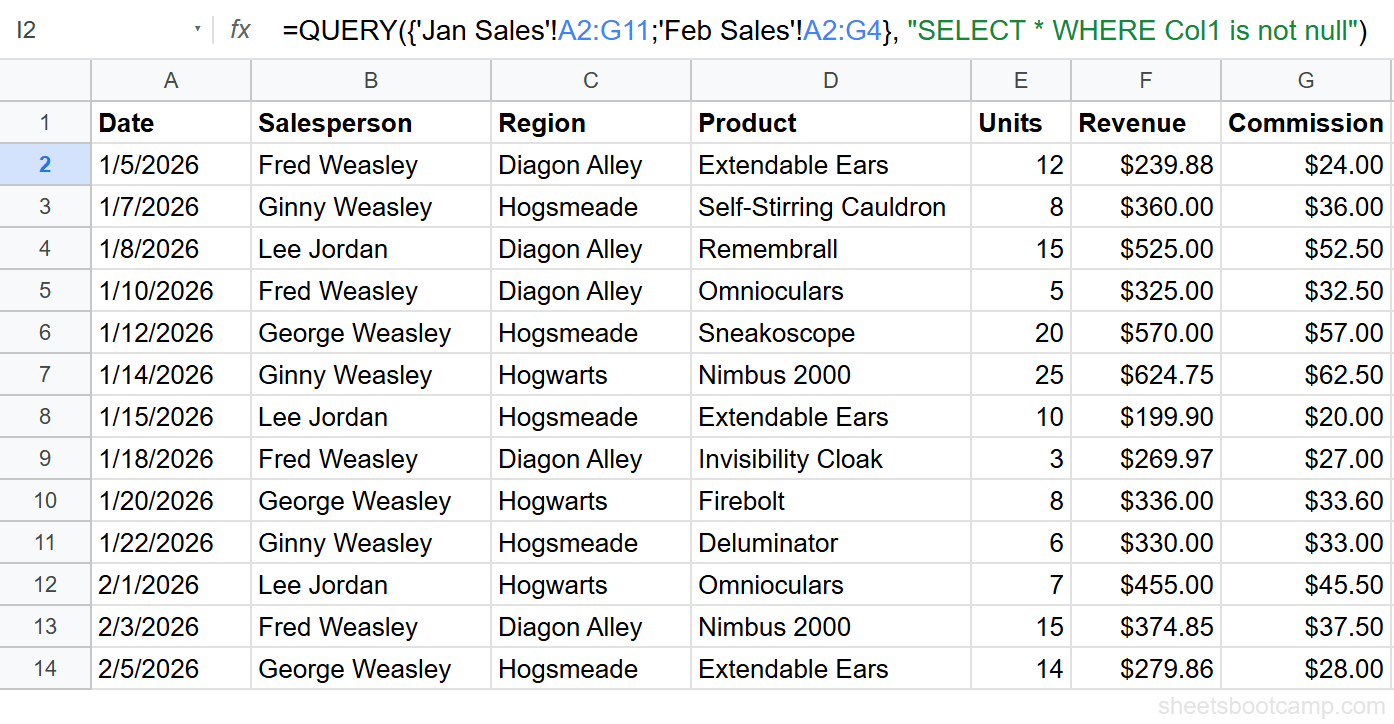
On a third sheet, enter:
=QUERY({'Jan Sales'!A2:G11;'Feb Sales'!A2:G4}, "SELECT * WHERE Col1 is not null")This stacks January and February data into one 13-row dataset (skipping headers from both sheets). The WHERE Col1 is not null filter removes any empty rows that appear when a range is larger than the actual data.
Filter the combined data
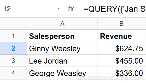
Enter:
=QUERY({'Jan Sales'!A2:G11;'Feb Sales'!A2:G4}, "SELECT Col2, Col6 WHERE Col3 = 'Hogwarts' ORDER BY Col6 DESC")This filters the combined 13-row dataset for Hogwarts transactions and returns Salesperson and Revenue, sorted by revenue descending. Three rows match: Ginny Weasley ($624.75), Lee Jordan ($455.00), and George Weasley ($336.00).
Add WHERE Col1 is not null to every combined-range QUERY. Open-ended ranges like A2:G may include blank rows that show up as empty results without this filter.
Col1, Col2 Notation
When QUERY operates on a combined array (curly braces), column letters are not available. Use Col1, Col2, etc. instead:
| Original Column | Col Reference | Header |
|---|---|---|
| A (Date) | Col1 | Date |
| B (Salesperson) | Col2 | Salesperson |
| C (Region) | Col3 | Region |
| D (Product) | Col4 | Product |
| E (Units) | Col5 | Units |
| F (Revenue) | Col6 | Revenue |
| G (Commission) | Col7 | Commission |
Mixing up Col notation is the most common error with combined ranges. Col6 in the combined array corresponds to column F in the original data. Map your columns carefully before writing the query string.
Combine Ranges from Different Sheets
The pattern for two sheets:
=QUERY({'Sheet1'!A2:G;'Sheet2'!A2:G}, "SELECT Col2, Col4, Col6 WHERE Col1 is not null")For three or more sheets, add more ranges separated by semicolons:
=QUERY({'Jan'!A2:G;'Feb'!A2:G;'Mar'!A2:G}, "SELECT * WHERE Col1 is not null")This stacks January, February, and March data into one QUERY. All ranges must have the same number of columns (7 in this example).
Filter and Sort Combined Data
All standard QUERY clauses work on combined ranges. Use Col notation instead of column letters:
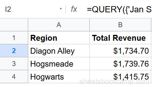
=QUERY({'Jan Sales'!A2:G11;'Feb Sales'!A2:G4}, "SELECT Col3, SUM(Col6) WHERE Col1 is not null GROUP BY Col3 ORDER BY SUM(Col6) DESC LABEL SUM(Col6) 'Total Revenue'")This groups the combined 13-row dataset by Region, sums Revenue, and sorts descending. GROUP BY, WHERE, ORDER BY, and LABEL all work the same way — you only change the column references from letters to Col numbers.
Combine with IMPORTRANGE
To QUERY data from a different spreadsheet, combine IMPORTRANGE with curly braces:
=QUERY({IMPORTRANGE("spreadsheet_url", "Sheet1!A2:G")}, "SELECT Col2, Col6 WHERE Col1 is not null")You can also mix local data with imported data:
=QUERY({A2:G11;IMPORTRANGE("spreadsheet_url", "Sheet1!A2:G")}, "SELECT * WHERE Col1 is not null")This stacks your local data with data from another spreadsheet into one QUERY. For a full guide on combining these functions, see QUERY with IMPORTRANGE.
You must grant access to the external spreadsheet before IMPORTRANGE works inside QUERY. Enter the IMPORTRANGE formula alone first to trigger the access prompt, then build the QUERY around it. See IMPORTRANGE Access Permission for details.
Common Mistakes
Using A, B, C instead of Col1, Col2, Col3
SELECT A, B causes a parse error on combined ranges. QUERY does not recognize column letters when the data source is a curly-brace array. Use SELECT Col1, Col2 instead.
Mismatched column counts
{'Jan Sales'!A2:G;'Feb Sales'!A2:F} fails because the first range has 7 columns and the second has 6. All stacked ranges must have the same number of columns.
Including headers from both sheets
{'Jan Sales'!A1:G;'Feb Sales'!A1:G} duplicates the header row. Start each range at row 2 to skip headers: {'Jan Sales'!A2:G;'Feb Sales'!A2:G}.
Missing WHERE Col1 is not null
Open-ended ranges (like A2:G without a row limit) include blank rows at the bottom. Without the null filter, your results show empty rows. Always add WHERE Col1 is not null.
Tips
1. Map your columns before writing the query. Write down which Col number corresponds to which header. This prevents the most common errors when working with combined ranges.
2. Test each range separately first. Run =QUERY('Jan Sales'!A2:G11, "SELECT *") alone to confirm the data looks right. Then combine ranges. Debugging is easier when you know each source is correct.
3. Use named ranges for readability. Instead of 'Jan Sales'!A2:G11, create a named range like JanData. The formula becomes =QUERY({JanData;FebData}, "SELECT * WHERE Col1 is not null"), which is easier to read and maintain.
For combining data from an external spreadsheet, see QUERY with IMPORTRANGE. For pulling data without querying it, see the IMPORTRANGE guide.
Related Google Sheets Tutorials
- QUERY Function: Complete Guide — covers all QUERY clauses with syntax and examples
- QUERY WHERE Clause — filter rows with conditions on the combined dataset
- QUERY with IMPORTRANGE — query data from external spreadsheets
- IMPORTRANGE Function — pull data from other spreadsheets without QUERY
Frequently Asked Questions
How do you QUERY multiple ranges in Google Sheets?
Use curly braces to stack ranges vertically: =QUERY({Sheet1!A2:C10;Sheet2!A2:C10}, "SELECT * WHERE Col1 is not null"). The semicolon stacks rows. All ranges must have the same number of columns.
Can you QUERY data from two different sheets?
Yes. Reference each sheet by name inside curly braces: {'Sheet1'!A2:C;'Sheet2'!A2:C}. Use Col1, Col2, Col3 notation instead of A, B, C because the combined range does not have standard column letters.
Why does QUERY use Col1 instead of A when combining ranges?
When you combine ranges with curly braces, the result is an array that has no column letters. QUERY references these columns as Col1, Col2, Col3. Using A, B, C causes a parse error on combined ranges.
How do you combine ranges vertically vs horizontally in QUERY?
Semicolons stack ranges vertically (adding rows): {A1:B5;A8:B12}. Commas place ranges side by side (adding columns): {A1:B5,D1:E5}. For QUERY across multiple sheets, vertical stacking with semicolons is the standard approach.
How do you handle headers when combining ranges in QUERY?
Start each range at row 2 to skip headers (Sheet1!A2:C, Sheet2!A2:C). Then either add a header manually above the QUERY output or use LABEL in the query string. Including headers from both sheets would create duplicate header rows in the combined data.