QUERY PIVOT in Google Sheets (Pivot-Style Reports)
Learn how to use QUERY PIVOT in Google Sheets to create cross-tabulated reports. Syntax, step-by-step examples, and tips for pivot-style summaries.
Sheets Bootcamp
May 1, 2026
QUERY PIVOT in Google Sheets turns unique values from one column into separate column headers, creating a cross-tabulated report inside a QUERY formula. It works like a formula-based pivot table — rows represent one dimension, columns represent another, and the cells contain aggregated values. We’ll cover the syntax, walk through building pivot reports, and show how PIVOT combines with WHERE and GROUP BY.
In This Guide
- PIVOT Syntax
- How to Create a QUERY PIVOT: Step-by-Step
- PIVOT with COUNT
- PIVOT with AVG
- PIVOT with WHERE (Filter Before Pivoting)
- QUERY PIVOT vs Pivot Tables
- Common Mistakes
- Tips
- Related Google Sheets Tutorials
- FAQ
PIVOT Syntax
PIVOT goes after GROUP BY in the query string:
=QUERY(data, "SELECT groupColumn, AGGREGATE(valueColumn) GROUP BY groupColumn PIVOT pivotColumn")| Part | Role | Example |
|---|---|---|
groupColumn | Becomes the row labels | B (Salesperson) |
AGGREGATE(valueColumn) | The calculation in each cell | SUM(F) (total Revenue) |
pivotColumn | Unique values become column headers | C (Region) |
PIVOT requires GROUP BY. The grouped column provides row labels, the aggregated column provides cell values, and the pivot column provides new column headers. All three pieces are required.
How to Create a QUERY PIVOT: Step-by-Step
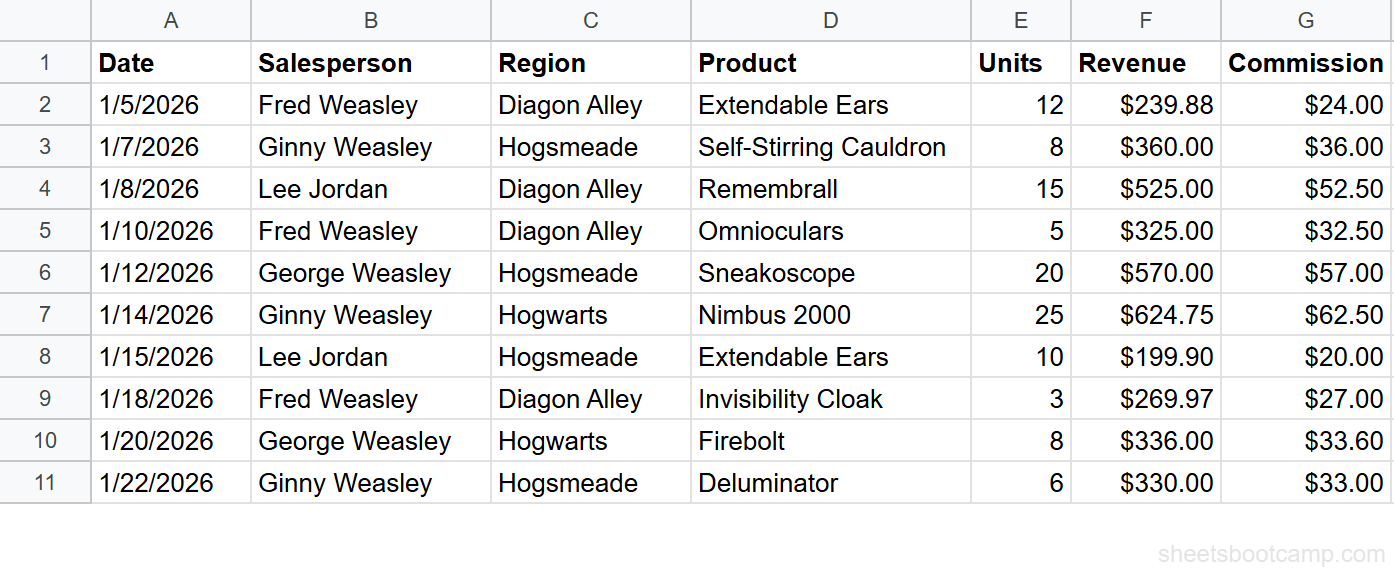
We’ll use the same sales records table from the QUERY guide. The data is in A1:G11 with 10 transactions.
Sample Data
| A | B | C | D | E | F | G | |
|---|---|---|---|---|---|---|---|
| 1 | Date | Salesperson | Region | Product | Units | Revenue | Commission |
| 2 | 1/5/2026 | Fred Weasley | Diagon Alley | Extendable Ears | 12 | $239.88 | $24.00 |
| 3 | 1/7/2026 | Ginny Weasley | Hogsmeade | Self-Stirring Cauldron | 8 | $360.00 | $36.00 |
| 4 | 1/8/2026 | Lee Jordan | Diagon Alley | Remembrall | 15 | $525.00 | $52.50 |
| 5 | 1/10/2026 | Fred Weasley | Diagon Alley | Omnioculars | 5 | $325.00 | $32.50 |
| 6 | 1/12/2026 | George Weasley | Hogsmeade | Sneakoscope | 20 | $570.00 | $57.00 |
| 7 | 1/14/2026 | Ginny Weasley | Hogwarts | Nimbus 2000 | 25 | $624.75 | $62.50 |
| 8 | 1/15/2026 | Lee Jordan | Hogsmeade | Extendable Ears | 10 | $199.90 | $20.00 |
| 9 | 1/18/2026 | Fred Weasley | Diagon Alley | Invisibility Cloak | 3 | $269.97 | $27.00 |
| 10 | 1/20/2026 | George Weasley | Hogwarts | Firebolt | 8 | $336.00 | $33.60 |
| 11 | 1/22/2026 | Ginny Weasley | Hogsmeade | Deluminator | 6 | $330.00 | $33.00 |
Review your data range
Your data lives in A1:G11. Row 1 is the header. You want to see total revenue per salesperson, broken down by region — a cross-tabulation with salespeople as rows and regions as columns.
Create a basic PIVOT
Select an empty cell and enter:
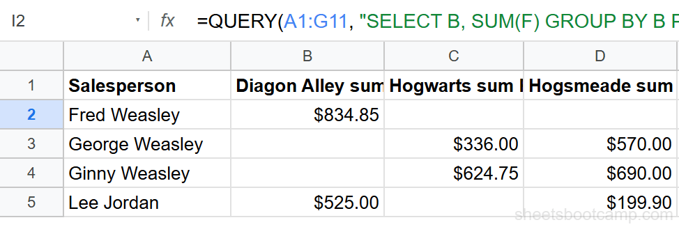
=QUERY(A1:G11, "SELECT B, SUM(F) GROUP BY B PIVOT C")QUERY groups by Salesperson (B), sums Revenue (F), and pivots on Region (C). The result has four columns: Salesperson, then one column for each unique region (Diagon Alley, Hogwarts, Hogsmeade). Fred Weasley’s Diagon Alley total is $834.85, and cells where a salesperson has no transactions in a region are left blank.
Add WHERE to filter before pivoting
Enter:
=QUERY(A1:G11, "SELECT B, SUM(F) WHERE F > 200 GROUP BY B PIVOT C")This filters out Lee Jordan’s $199.90 Hogsmeade transaction before creating the pivot. Lee Jordan’s Hogsmeade column is now blank because his only Hogsmeade transaction was below $200.
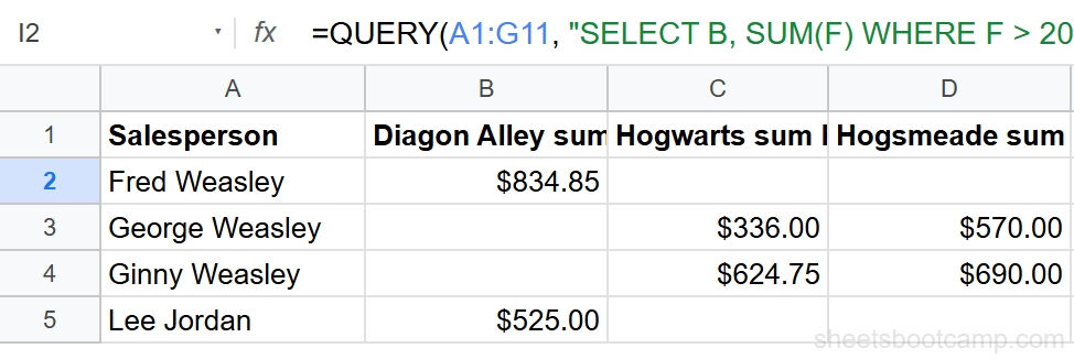
WHERE runs before GROUP BY and PIVOT. Use it to exclude outliers or irrelevant rows from your summary before the cross-tabulation is built.
PIVOT with COUNT
COUNT counts the number of transactions instead of summing values:
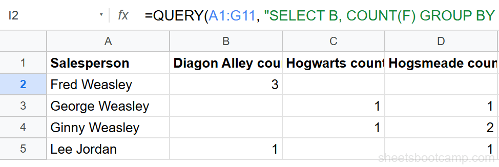
=QUERY(A1:G11, "SELECT B, COUNT(F) GROUP BY B PIVOT C")This shows how many transactions each salesperson made in each region. Fred Weasley has 3 transactions in Diagon Alley, 0 in Hogwarts, and 0 in Hogsmeade.
PIVOT with AVG
AVG calculates the average value per cell:
=QUERY(A1:G11, "SELECT B, AVG(F) GROUP BY B PIVOT C")This returns the average revenue per transaction for each salesperson-region combination. George Weasley’s average in Hogsmeade is $570.00 (one transaction), while his Hogwarts average is $336.00.
QUERY PIVOT vs Pivot Tables
Both create cross-tabulated summaries, but they work differently:
| Feature | QUERY PIVOT | Pivot Table |
|---|---|---|
| Output location | In the same sheet as a formula | Separate sheet or overlay |
| Auto-updates | Yes, on data change | Yes, on refresh |
| Combines with filters | WHERE in same formula | Separate filter controls |
| Multiple aggregates | One per formula | Multiple in one pivot |
| Custom formulas | Full QUERY syntax | Limited calculated fields |
| Learning curve | Text-based query string | Point-and-click editor |
Use QUERY PIVOT when you want a formula-driven summary that stays on the same sheet. Use a pivot table when you need interactive slicing, multiple aggregations, or a point-and-click interface.
Common Mistakes
Missing GROUP BY
PIVOT requires GROUP BY. SELECT B, SUM(F) PIVOT C without GROUP BY causes a parse error. The GROUP BY column provides the row labels for the pivot.
Trying to use LABEL with PIVOT headers
LABEL cannot rename the auto-generated PIVOT column headers. PIVOT creates headers from the unique values in the pivot column (like “Diagon Alley sum Revenue”). To rename them, add a header row manually above the QUERY output.
Using multiple aggregates
QUERY PIVOT supports one aggregate function per formula. SELECT B, SUM(F), COUNT(F) GROUP BY B PIVOT C causes an error. Run two separate QUERY formulas for SUM and COUNT.
Putting PIVOT before GROUP BY
Clause order is fixed: SELECT, WHERE, GROUP BY, PIVOT, ORDER BY, LIMIT. PIVOT must come after GROUP BY.
Tips
1. PIVOT column order follows the order values appear in the data. If regions appear as Diagon Alley, Hogsmeade, Hogwarts in the data, those become the column order. To change the order, sort your source data first or use ORDER BY on the grouped column.
2. Blank cells in the pivot result mean no matching data exists. Fred Weasley has no Hogwarts transactions, so that cell is empty. If you need zeros instead of blanks, wrap individual cells in IFERROR or post-process the result.
3. PIVOT works on any column with a manageable number of unique values. A column with 3 regions creates 3 extra columns. A column with 100 products creates 100 columns. Keep the pivot column to a reasonable number of categories.
PIVOT and GROUP BY can use different columns. GROUP BY defines the rows, PIVOT defines the columns. The aggregate function fills the intersection of each row and column.
Related Google Sheets Tutorials
- QUERY Function: Complete Guide — covers all QUERY clauses with syntax and examples
- QUERY GROUP BY — aggregate data without cross-tabulation
- QUERY ORDER BY — sort QUERY results ascending or descending
- Pivot Tables Guide — interactive pivot tables for point-and-click analysis
Frequently Asked Questions
What does PIVOT do in QUERY in Google Sheets?
PIVOT rotates unique values from one column into new column headers. Combined with an aggregate function like SUM or COUNT, it creates a cross-tabulated summary where rows represent one dimension and columns represent another.
What is the difference between QUERY PIVOT and a pivot table?
QUERY PIVOT is a formula that returns a live, cross-tabulated result directly in your sheet. A pivot table is a separate interactive object with its own editor. QUERY PIVOT updates automatically when source data changes and can be combined with WHERE and ORDER BY in the same formula.
Can you use PIVOT with multiple aggregate functions?
No. QUERY PIVOT supports only one aggregate function per formula. To show both SUM and COUNT, you need two separate QUERY formulas. GROUP BY supports multiple aggregates in one formula but produces a different output layout.
How do you rename PIVOT column headers in QUERY?
PIVOT auto-generates headers from the pivot column values (like Diagon Alley, Hogwarts, Hogsmeade). You cannot use LABEL to rename PIVOT headers directly. To rename them, wrap the QUERY in a second formula or manually adjust the headers.
Can you combine QUERY PIVOT with WHERE?
Yes. WHERE filters the data before PIVOT creates the cross-tabulation. For example: SELECT B, SUM(F) WHERE F > 200 GROUP BY B PIVOT C returns only transactions with revenue over $200, then pivots by region.