QUERY SELECT in Google Sheets: Choose Columns
Learn how to use QUERY SELECT in Google Sheets to pick specific columns, reorder them, and use aggregate functions. Step-by-step examples and syntax.
Sheets Bootcamp
March 1, 2026
QUERY SELECT in Google Sheets controls which columns appear in the output. Instead of returning all seven columns from a data range, you pick the two or three you need. It is the first clause in every QUERY formula and the foundation for everything else QUERY does. We’ll cover column selection, reordering, using SELECT *, and combining SELECT with aggregate functions.
In This Guide
- SELECT Syntax
- How to Use QUERY SELECT: Step-by-Step
- Select All Columns with SELECT *
- Reorder Columns
- SELECT with Aggregate Functions
- SELECT with Other Clauses
- Common Mistakes
- Tips
- Related Google Sheets Tutorials
- FAQ
SELECT Syntax
SELECT is the first clause in a QUERY string. List column letters separated by commas:
=QUERY(data, "SELECT column1, column2, column3")| Pattern | What It Does |
|---|---|
SELECT A, B, C | Returns columns A, B, and C |
SELECT * | Returns all columns |
SELECT F, B | Returns columns F and B in that order |
SELECT B, SUM(F) | Returns column B and the sum of column F (requires GROUP BY) |
Column letters must match the columns in your data range. If your data starts in column A, then A in the query is the first column. If your data starts in column D, then D in the query is the first column.
Column letters in SELECT refer to the columns in your data range, not the spreadsheet. If your QUERY range is D1:H11, then D is the first column in the query — not A.
How to Use QUERY SELECT: Step-by-Step
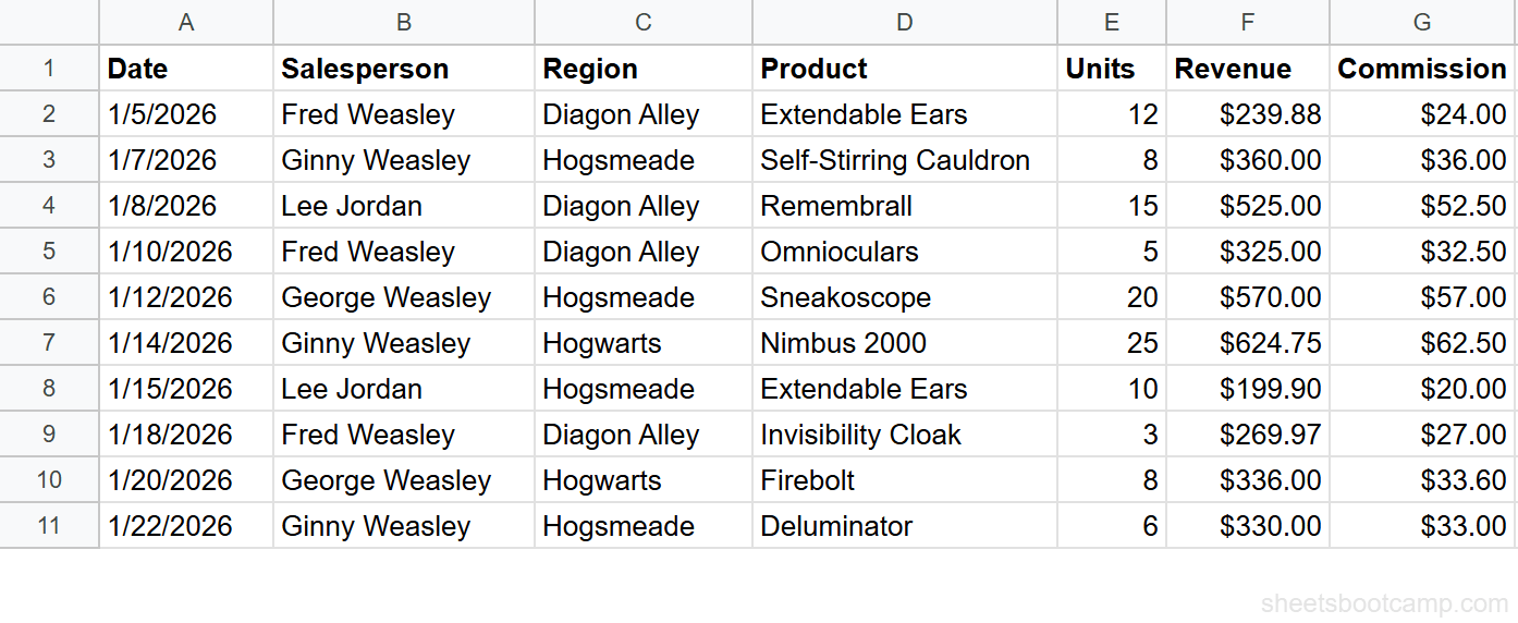
We’ll use the same sales records table from the QUERY guide. The data is in A1:G11 with 10 transactions.
Sample Data
| A | B | C | D | E | F | G | |
|---|---|---|---|---|---|---|---|
| 1 | Date | Salesperson | Region | Product | Units | Revenue | Commission |
| 2 | 1/5/2026 | Fred Weasley | Diagon Alley | Extendable Ears | 12 | $239.88 | $24.00 |
| 3 | 1/7/2026 | Ginny Weasley | Hogsmeade | Self-Stirring Cauldron | 8 | $360.00 | $36.00 |
| 4 | 1/8/2026 | Lee Jordan | Diagon Alley | Remembrall | 15 | $525.00 | $52.50 |
| 5 | 1/10/2026 | Fred Weasley | Diagon Alley | Omnioculars | 5 | $325.00 | $32.50 |
| 6 | 1/12/2026 | George Weasley | Hogsmeade | Sneakoscope | 20 | $570.00 | $57.00 |
| 7 | 1/14/2026 | Ginny Weasley | Hogwarts | Nimbus 2000 | 25 | $624.75 | $62.50 |
| 8 | 1/15/2026 | Lee Jordan | Hogsmeade | Extendable Ears | 10 | $199.90 | $20.00 |
| 9 | 1/18/2026 | Fred Weasley | Diagon Alley | Invisibility Cloak | 3 | $269.97 | $27.00 |
| 10 | 1/20/2026 | George Weasley | Hogwarts | Firebolt | 8 | $336.00 | $33.60 |
| 11 | 1/22/2026 | Ginny Weasley | Hogsmeade | Deluminator | 6 | $330.00 | $33.00 |
Review your data range
Your data is in A1:G11. Row 1 is the header. Seven columns: Date (A), Salesperson (B), Region (C), Product (D), Units (E), Revenue (F), and Commission (G).
Select specific columns
Select an empty cell and enter:
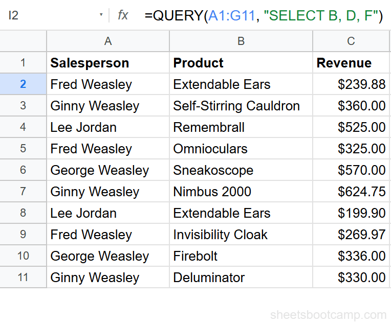
=QUERY(A1:G11, "SELECT B, D, F")This returns a new table with three columns: Salesperson, Product, and Revenue. The header row carries over automatically. All 10 data rows appear because there is no WHERE filter.
Reorder columns in the output
Enter:
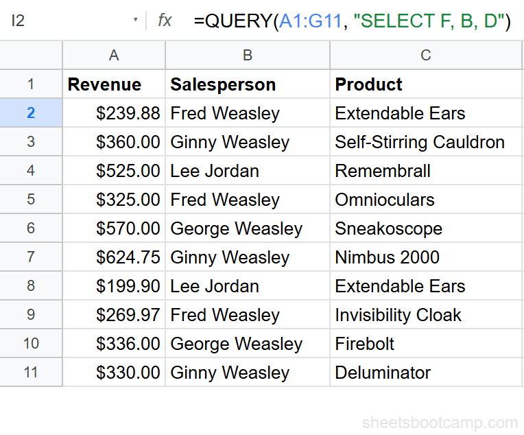
=QUERY(A1:G11, "SELECT F, B, D")This returns the same three columns, but Revenue appears first, followed by Salesperson and Product. The output order matches your SELECT order.
QUERY SELECT is the fastest way to restructure a table without copying data. You get a new view of your data that updates automatically when the source changes.
Select All Columns with SELECT *
The asterisk returns every column:
=QUERY(A1:G11, "SELECT *")This is equivalent to =QUERY(A1:G11, "SELECT A, B, C, D, E, F, G"). It is useful when you want all columns but plan to add a WHERE filter, ORDER BY, or LIMIT clause:
=QUERY(A1:G11, "SELECT * ORDER BY F DESC")This returns all columns, sorted by Revenue from highest to lowest.
You cannot mix * with specific column letters. SELECT *, B is not valid. Use either * for everything or list the exact columns you want.
Reorder Columns
SELECT returns columns in the order you list them. This lets you rearrange a table without touching the original data:
=QUERY(A1:G11, "SELECT C, B, F, D")This returns Region, Salesperson, Revenue, Product — completely different from the original column order. The source data stays unchanged.
You can also repeat a column if needed for layout purposes:
=QUERY(A1:G11, "SELECT B, F, B")This returns Salesperson, Revenue, and Salesperson again. Google Sheets appends a number to duplicate headers (e.g., “Salesperson1”) to keep them unique.
SELECT with Aggregate Functions
When paired with GROUP BY, SELECT can include aggregate functions:
| Function | What It Does |
|---|---|
SUM(col) | Adds all values in the column |
COUNT(col) | Counts non-empty cells |
AVG(col) | Calculates the average |
MIN(col) | Returns the smallest value |
MAX(col) | Returns the largest value |
SUM Example
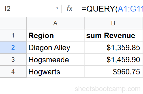
=QUERY(A1:G11, "SELECT C, SUM(F) GROUP BY C")This returns one row per region with the total revenue. Diagon Alley: $1,359.85. Hogsmeade: $1,459.90. Hogwarts: $960.75.
COUNT Example
=QUERY(A1:G11, "SELECT B, COUNT(D) GROUP BY B")This counts the number of transactions per salesperson. Fred Weasley: 3. Ginny Weasley: 3. George Weasley: 2. Lee Jordan: 2.
Multiple Aggregations
You can include several aggregate functions in a single SELECT:
=QUERY(A1:G11, "SELECT C, SUM(F), AVG(F), COUNT(F) GROUP BY C")This returns the total, average, and count of revenue per region in one table.
Every non-aggregated column in SELECT must appear in GROUP BY. If you write SELECT B, C, SUM(F) GROUP BY C, the query breaks because B is not aggregated or grouped. Either add B to GROUP BY or remove it from SELECT.
SELECT with Other Clauses
SELECT pairs with every other QUERY clause. The clauses must follow this order: SELECT, WHERE, GROUP BY, PIVOT, ORDER BY, LIMIT, OFFSET, LABEL, FORMAT.
SELECT + WHERE
=QUERY(A1:G11, "SELECT B, F WHERE F > 400")Returns Salesperson and Revenue, but only for transactions over $400. See the QUERY WHERE guide for more filtering patterns.
SELECT + ORDER BY
=QUERY(A1:G11, "SELECT B, D, F ORDER BY F DESC")Returns three columns, sorted by Revenue from highest to lowest.
SELECT + LIMIT
=QUERY(A1:G11, "SELECT B, F ORDER BY F DESC LIMIT 3")Returns the top 3 transactions by revenue.
SELECT + LABEL
=QUERY(A1:G11, "SELECT C, SUM(F) GROUP BY C LABEL SUM(F) 'Total Revenue'")Renames the aggregated column header from “sum Revenue” to “Total Revenue”. See the QUERY GROUP BY guide for more aggregation patterns.
Common Mistakes
Referencing a column outside the data range
If your data is in A1:D11, you cannot use SELECT F — column F is not in the range. QUERY returns a parsing error. Match your column letters to the range you provide.
Using column names instead of letters
SELECT Revenue does not work. QUERY uses column letters: SELECT F. Column letters correspond to positions in your data range, not header text.
Mixing * with specific columns
SELECT *, F is invalid syntax. Use SELECT * alone for all columns. If you want all columns plus a calculated column, you need to list every column letter individually.
Forgetting GROUP BY with aggregate functions
SELECT C, SUM(F) without GROUP BY returns an error. Any time you use SUM, COUNT, AVG, MIN, or MAX in SELECT, you need a GROUP BY clause for the non-aggregated columns.
Tips
1. Use SELECT to create clean reporting views. Instead of hiding columns or copying data, a QUERY SELECT formula gives you a live, filtered view that updates when the source data changes.
2. Combine with LABEL to rename headers. The default aggregation headers (like “sum Revenue”) are not readable. Use LABEL to rename them: LABEL SUM(F) 'Total Revenue'.
3. Pair SELECT with VLOOKUP for two-step lookups. QUERY SELECT can extract a subset of columns, then VLOOKUP can search that result. This is useful when you need to narrow a large dataset before looking up a specific value.
When building a QUERY formula, start with SELECT * and add clauses one at a time. Once the results look right, narrow the SELECT to only the columns you need. This makes debugging faster.
Related Google Sheets Tutorials
- QUERY Function: Complete Guide — covers all QUERY clauses with syntax and examples
- QUERY WHERE Clause — filter rows using conditions, comparisons, and text matching
- QUERY GROUP BY — summarize and aggregate data with SUM, COUNT, and AVG
- VLOOKUP Complete Guide — look up values from a table when you need a single value instead of a column view
Frequently Asked Questions
How do you select specific columns with QUERY in Google Sheets?
Use the SELECT clause with column letters separated by commas. For example, =QUERY(A1:G11, "SELECT B, D, F") returns only the Salesperson, Product, and Revenue columns from a 7-column data range.
Can you reorder columns with QUERY SELECT?
Yes. List the columns in the order you want them. =QUERY(A1:G11, "SELECT F, B, D") returns Revenue first, then Salesperson, then Product. The output order matches your SELECT order, not the original data order.
What does SELECT * mean in QUERY?
SELECT * returns all columns from the data range. It is the default if you omit the SELECT clause entirely. Use it when you want all columns but need a WHERE filter, ORDER BY, or LIMIT.
Can you use SELECT with aggregate functions?
Yes. SELECT works with SUM, COUNT, AVG, MIN, and MAX when combined with GROUP BY. For example, =QUERY(A1:G11, "SELECT C, SUM(F) GROUP BY C") returns one row per region with the total revenue.