LEFT, RIGHT, MID Functions in Google Sheets
Learn how to extract text with LEFT, RIGHT, and MID in Google Sheets. Pull characters from the start, end, or middle of any cell with step-by-step examples.
Sheets Bootcamp
March 24, 2026
LEFT, RIGHT, and MID in Google Sheets extract a specific number of characters from a text string. LEFT pulls from the start, RIGHT pulls from the end, and MID pulls from any position in the middle. The text functions guide covers the full set of text tools, and these three extraction functions are among the most used.
This guide covers the syntax for each function, how to combine them with FIND for dynamic extraction, and step-by-step examples using real data.
In This Guide
- LEFT Function
- RIGHT Function
- MID Function
- Extract Text Step-by-Step
- Dynamic Extraction with FIND
- Practical Examples
- Common Errors and How to Fix Them
- Tips and Best Practices
- Related Google Sheets Tutorials
- Frequently Asked Questions
LEFT Function
LEFT returns the first N characters from a text string.
=LEFT(text, [num_characters])| Argument | Description | Required |
|---|---|---|
| text | The text string or cell reference | Yes |
| num_characters | How many characters to extract (default: 1) | No |
Example: =LEFT("HARRY POTTER", 5) returns "HARRY". If you omit the second argument, =LEFT(A2) returns only the first character.
LEFT counts every character, including spaces. =LEFT(" Ronald Weasley ", 5) returns " Ron" because the two leading spaces count as characters.
RIGHT Function
RIGHT returns the last N characters from a text string.
=RIGHT(text, [num_characters])| Argument | Description | Required |
|---|---|---|
| text | The text string or cell reference | Yes |
| num_characters | How many characters to extract (default: 1) | No |
Example: =RIGHT("GU1 1AA", 3) returns "1AA". =RIGHT(D2, 7) returns the last 7 characters of the address, which is the postal code.
RIGHT is useful for extracting fixed-length codes from the end of strings: postal codes, file extensions, or suffix identifiers.
MID Function
MID returns characters from any position in a text string.
=MID(text, start_position, num_characters)| Argument | Description | Required |
|---|---|---|
| text | The text string or cell reference | Yes |
| start_position | Position to start extracting (1 = first character) | Yes |
| num_characters | How many characters to extract | Yes |
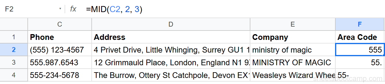
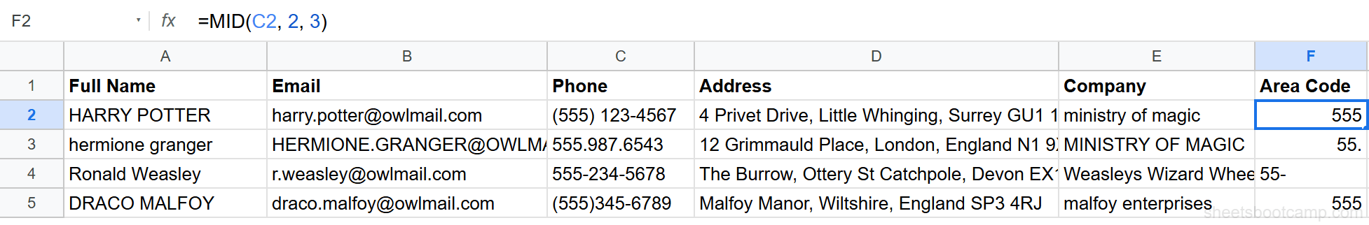
Example: =MID("(555) 123-4567", 2, 3) starts at position 2 and extracts 3 characters, returning "555". Position 1 is the opening parenthesis, so position 2 is the first digit.
Positions in Google Sheets text functions start at 1, not 0. The first character is position 1, the second is position 2, and so on. This is different from programming languages that use zero-based indexing.
Extract Text Step-by-Step
We’ll extract area codes, postal codes, and first names from the messy contacts table.
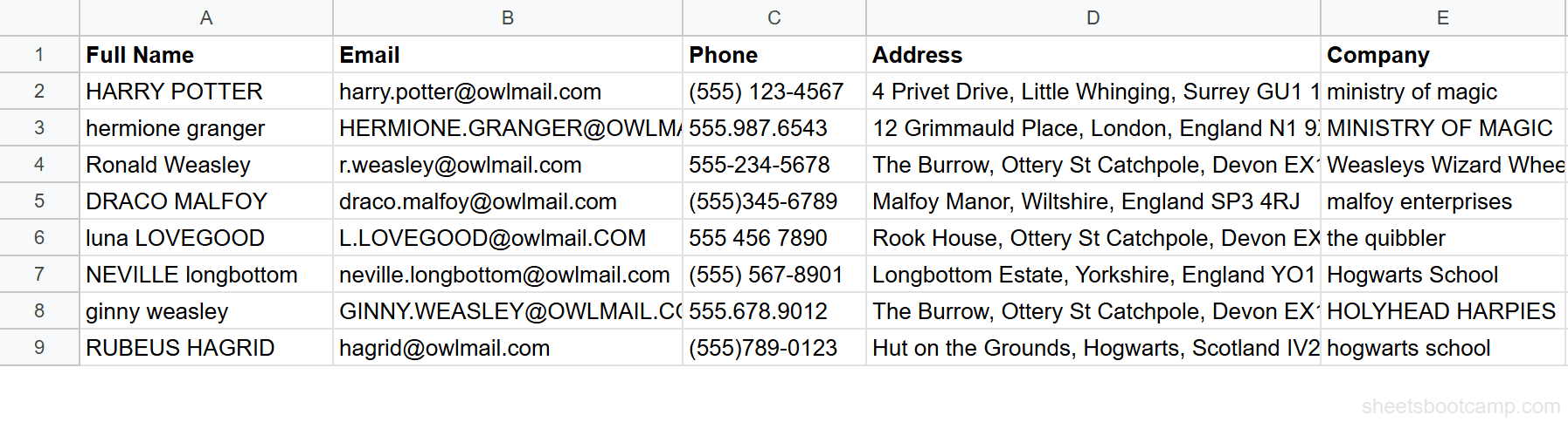
Set up your data
Open the contacts spreadsheet. Column C has phone numbers in mixed formats: "(555) 123-4567", "555.987.6543", "555-234-5678", and "(555)345-6789". Column D has full addresses ending in postal codes. Column A has names with extra spaces.
Extract the area code with MID
For phone numbers starting with "(", the area code begins at position 2. Select cell F2 and enter:
=MID(C2, 2, 3)For "(555) 123-4567", this returns "555". Copy the formula down. For rows where the phone starts without parentheses (like "555.987.6543"), use =LEFT(C2, 3) instead. We’ll handle mixed formats in the examples section.
Extract the postal code with RIGHT
UK postal codes are 7 characters (including the space). Select cell G2 and enter:
=RIGHT(D2, 7)For "4 Privet Drive, Little Whinging, Surrey GU1 1AA", this returns "GU1 1AA". Copy the formula down through row 9. Every address in the data ends with a 7-character postal code, so RIGHT works consistently here.
Extract the first name with LEFT and FIND
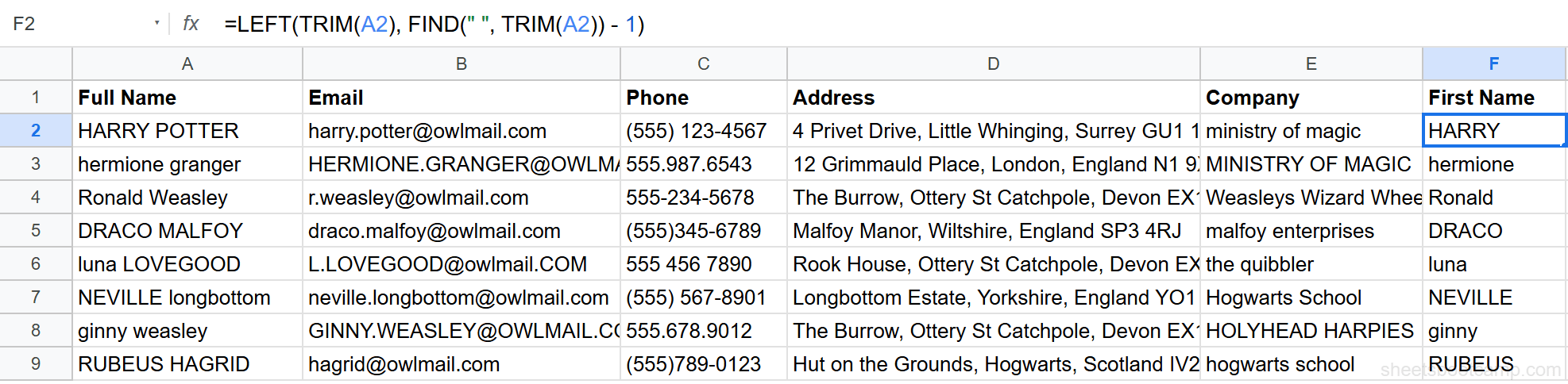
Select cell H2 and enter:
=LEFT(TRIM(A2), FIND(" ", TRIM(A2)) - 1)TRIM removes extra spaces first. Then FIND locates the first space. Subtracting 1 gives the length of the first name. LEFT extracts that many characters. For "HARRY POTTER" (after TRIM becomes "HARRY POTTER"), FIND returns 6, and LEFT returns the first 5 characters: "HARRY".
This formula breaks if the name has no space, like a single-word name. FIND returns an error when it cannot locate the search string. Wrap the formula in IFERROR to handle this: =IFERROR(LEFT(TRIM(A2), FIND(” ”, TRIM(A2)) - 1), TRIM(A2)). This returns the full name when no space exists.
Dynamic Extraction with FIND
Hardcoding the number of characters works when the length is fixed (area codes are always 3 digits, postal codes are always 7 characters). For variable-length text, combine LEFT, RIGHT, or MID with FIND to calculate positions dynamically.
Extract the Last Name
The last name is everything after the first space.
=MID(TRIM(A2), FIND(" ", TRIM(A2)) + 1, LEN(TRIM(A2)))FIND locates the space. Adding 1 moves past it. MID extracts from that position through the end of the string. Using LEN as the num_characters argument is safe because MID stops at the end of the text even if the count exceeds the remaining characters.
Extract the Username from an Email
The username is everything before the @ symbol.
=LEFT(B2, FIND("@", B2) - 1)For "harry.potter@owlmail.com", FIND returns 13 (the position of @), and LEFT returns the first 12 characters: "harry.potter".
Extract the Domain from an Email
The domain is everything after the @ symbol.
=MID(B2, FIND("@", B2) + 1, LEN(B2))For the same email, this returns "owlmail.com".
Practical Examples
Example 1: Handle Mixed Phone Formats
The contacts have phones in 4 formats. To extract the 10-digit number regardless of format, strip non-numeric characters first using SUBSTITUTE, then use LEFT and MID:
=LEFT(SUBSTITUTE(SUBSTITUTE(SUBSTITUTE(SUBSTITUTE(SUBSTITUTE(C2,"(",""),")",""),"-",""),".","")," ",""), 3)This strips all formatting and returns the first 3 digits (area code) from any format. Apply the same cleaning, then use MID(cleaned, 4, 3) for the exchange and RIGHT(cleaned, 4) for the last 4 digits.
Example 2: Extract Initials
To create initials from a name like "Harry Potter":
=LEFT(TRIM(A2), 1) & LEFT(MID(TRIM(A2), FIND(" ", TRIM(A2)) + 1, LEN(TRIM(A2))), 1)LEFT gets the first character of the first name. MID extracts the last name, then LEFT gets its first character. For "Harry Potter", this returns "HP".
Example 3: Get File Extension
If a cell contains a filename like "report.xlsx":
=RIGHT(A2, LEN(A2) - FIND(".", A2))FIND locates the dot. LEN minus the dot position gives the length of the extension. RIGHT extracts it. This returns "xlsx".
Common Errors and How to Fix Them
#VALUE! Error from MID Start Position
MID returns #VALUE! if start_position is less than 1 or num_characters is negative. This typically happens when a FIND-based calculation does not find the expected character. Check that the delimiter exists in the text before using it in a MID calculation.
FIND Not Finding the Character
=FIND(" ", A2) returns an error if A2 has no space. Always wrap FIND in IFERROR when the search character might not exist: =IFERROR(FIND(" ", A2), 0) returns 0 instead of an error.
LEFT/RIGHT Returning Spaces
If LEFT or RIGHT returns unexpected spaces, the source text has leading or trailing whitespace. Use TRIM to clean the text before extracting: =LEFT(TRIM(A2), 5).
Use LEN to count characters before extracting. =LEN(A2) shows the total character count, including invisible spaces. If the count is higher than expected, wrap the cell in TRIM first.
Tips and Best Practices
-
Combine with FIND for dynamic extraction. Hardcoded character counts break when data varies in length.
=LEFT(A2, FIND(" ", A2) - 1)adapts to any first name length. -
TRIM before extracting. Extra spaces change character positions and counts. Always TRIM the source text when working with imported or user-entered data.
-
MID with a large num_characters is safe.
=MID(A2, 5, 999)returns everything from position 5 to the end. MID does not error if the count exceeds the available characters — it returns what is available. -
Use SPLIT when the text has consistent delimiters. If you need the second word from a comma-separated string,
=INDEX(SPLIT(A2, ","), 1, 2)is cleaner than calculating positions with FIND and MID. -
FIND is case-sensitive, SEARCH is not. When locating a character for extraction, use FIND for exact case matches and SEARCH when case does not matter.
Related Google Sheets Tutorials
- Text Functions in Google Sheets — Full guide to cleaning, extracting, and combining text
- SPLIT Function in Google Sheets — Separate text into columns by delimiter instead of character position
- CONCATENATE and TEXTJOIN — Combine extracted text back into a single string
- TRIM and CLEAN in Google Sheets — Remove extra spaces before extracting text
- IF Function in Google Sheets — Conditional logic to handle different text patterns with LEFT, RIGHT, and MID
Frequently Asked Questions
How do I extract the first N characters from a cell in Google Sheets?
Use the LEFT function. =LEFT(A2, 5) returns the first 5 characters from cell A2. For "HARRY POTTER", this returns "HARRY". If you omit the second argument, LEFT returns only the first character.
How do I extract the last N characters from a cell in Google Sheets?
Use the RIGHT function. =RIGHT(A2, 6) returns the last 6 characters from cell A2. For the postal code "GU1 1AA" at the end of an address, =RIGHT(D2, 7) extracts it. If you omit the second argument, RIGHT returns only the last character.
How do I extract text from the middle of a cell in Google Sheets?
Use the MID function. =MID(A2, 3, 4) starts at position 3 and extracts 4 characters. For "(555) 123-4567" in a phone number cell, =MID(C2, 2, 3) starts at position 2 and pulls 3 characters, returning "555".
How do I extract the first name from a full name in Google Sheets?
Combine LEFT with FIND to locate the first space: =LEFT(A2, FIND(" ", A2) - 1). FIND returns the position of the first space, and subtracting 1 gives the length of the first name. For "Harry Potter", FIND returns 6, so LEFT returns the first 5 characters: "Harry".
What is the difference between MID and SPLIT for extracting text?
MID extracts a fixed number of characters from a known position. SPLIT divides text at a delimiter into separate cells. Use MID when you know exactly where the text starts and how long it is, like extracting an area code. Use SPLIT when the text has a consistent delimiter like a comma or space.