TRIM & CLEAN Functions in Google Sheets
Learn how to remove extra spaces and non-printable characters in Google Sheets with TRIM and CLEAN. Fix imported data, broken lookups, and whitespace issues.
Sheets Bootcamp
March 25, 2026
The TRIM function in Google Sheets removes extra spaces from text — leading spaces, trailing spaces, and repeated spaces between words. It is the most frequently used cleanup function because extra spaces are invisible yet break VLOOKUP, comparisons, and sorting. The text functions guide covers the full set of text tools, and TRIM is usually the first one you reach for on imported data.
This guide covers TRIM and CLEAN syntax, when to use each, how to handle non-breaking spaces, and why TRIM should be your first step with any imported data.
In This Guide
- TRIM Syntax and Examples
- CLEAN Syntax and Examples
- TRIM vs CLEAN: When to Use Each
- Remove Extra Spaces Step-by-Step
- Non-Breaking Spaces and CHAR(160)
- Practical Examples
- Common Errors and How to Fix Them
- Tips and Best Practices
- Related Google Sheets Tutorials
- Frequently Asked Questions
TRIM Syntax and Examples
=TRIM(text)| Argument | Description | Required |
|---|---|---|
| text | The text string or cell reference to clean | Yes |
TRIM does three things:
- Removes all leading spaces
- Removes all trailing spaces
- Collapses multiple consecutive spaces between words to a single space
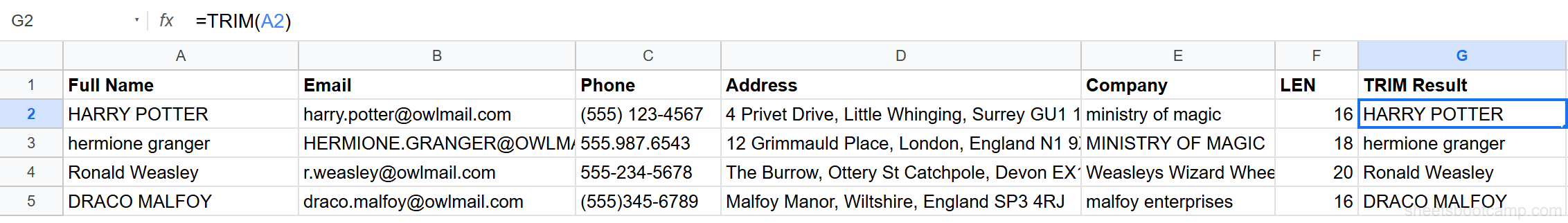
Example: =TRIM(" HARRY POTTER ") returns "HARRY POTTER". The two leading spaces, two trailing spaces, and two extra internal spaces are all removed.
Cell A3 in the contacts table contains " Ronald Weasley ". =TRIM(A3) returns "Ronald Weasley" with no extra spaces.
CLEAN Syntax and Examples
=CLEAN(text)| Argument | Description | Required |
|---|---|---|
| text | The text string or cell reference to clean | Yes |
CLEAN removes non-printable characters — characters with ASCII codes 0 through 31. These include:
- Line breaks (CHAR(10), CHAR(13))
- Tabs (CHAR(9))
- Control characters that appear when importing from web pages, databases, or external APIs
Example: If a cell displays "Harry Potter" but LEN returns 14 instead of 12, there are hidden characters. =CLEAN(A2) removes them. =LEN(CLEAN(A2)) returns the expected count.
CLEAN does not remove extra spaces. It handles only non-printable characters. To clean both invisible characters and spaces, combine them: =TRIM(CLEAN(A2)).
TRIM vs CLEAN: When to Use Each
| Problem | Function | Example |
|---|---|---|
| Extra spaces between words | TRIM | "HARRY POTTER" → "HARRY POTTER" |
| Leading/trailing spaces | TRIM | " Ronald " → "Ronald" |
| Line breaks in cells | CLEAN | Removes CHAR(10) and CHAR(13) |
| Tab characters | CLEAN | Removes CHAR(9) |
| Imported web data | Both | =TRIM(CLEAN(A2)) |
For data imported from web pages, CSV files, or external systems, always use =TRIM(CLEAN(A2)) as your default cleanup formula. Web data often contains both extra spaces and non-printable characters that are invisible in the cell but break formulas.
Remove Extra Spaces Step-by-Step
We’ll clean the names in the messy contacts table using TRIM and verify the results with LEN.
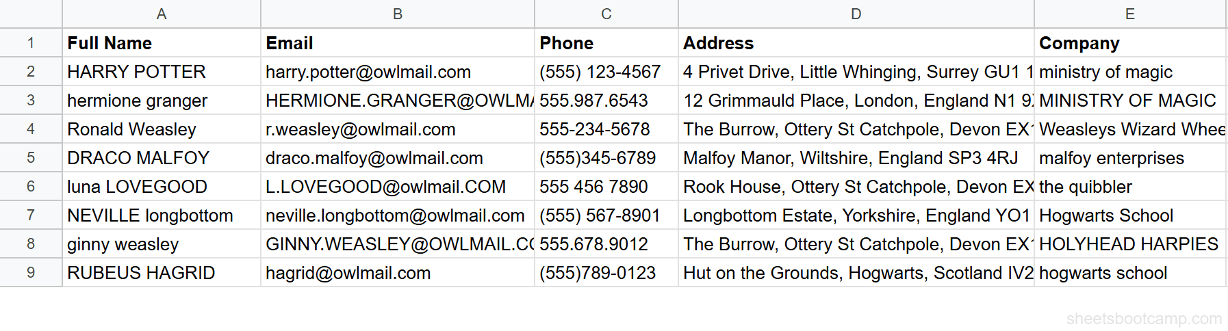
Identify the whitespace problems
Open the contacts spreadsheet. Column A has names with spacing issues:
| Row | Original Value | Visible Problem |
|---|---|---|
| 2 | "HARRY POTTER" | 3 spaces between words |
| 3 | "hermione granger" | Looks clean, but check with LEN |
| 4 | " Ronald Weasley " | Leading and trailing spaces |
| 6 | " NEVILLE longbottom " | Leading/trailing spaces plus mixed case |
| 10 | " Albus Dumbledore" | Leading spaces and extra internal space |
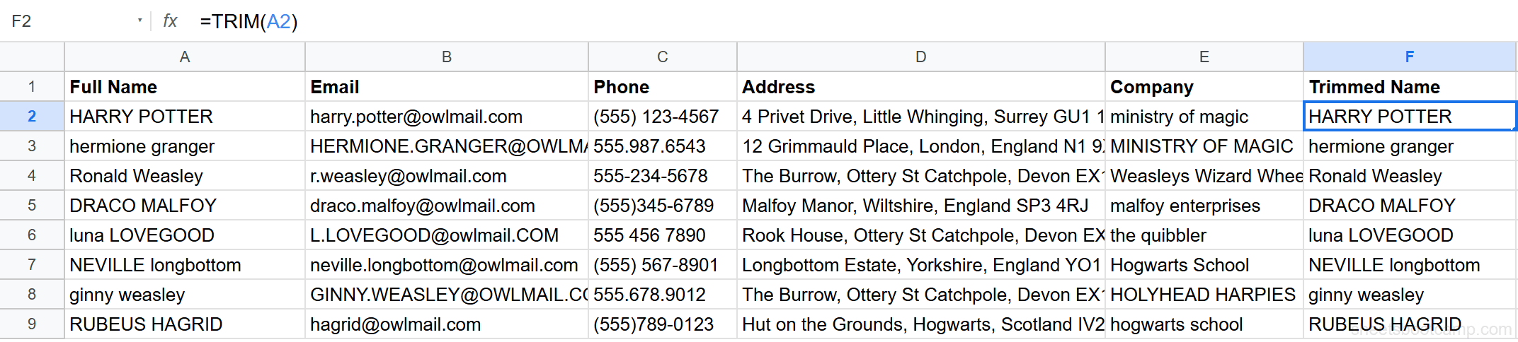
Apply TRIM to remove extra spaces
Select cell F2 and enter:
=TRIM(A2)For "HARRY POTTER", this returns "HARRY POTTER" with a single space. Copy the formula down through F9 for all 8 rows.
Use CLEAN for imported data
If you suspect non-printable characters (common with web-imported data), enter:
=TRIM(CLEAN(A2))This strips invisible characters first, then removes extra spaces. For the contacts data, CLEAN may not change anything visible, but it prevents future issues if the data was copy-pasted from a web source.
Make TRIM(CLEAN()) your default cleanup formula for any imported data. Even if the data looks fine, invisible characters can cause lookups to fail silently — the values appear identical but Google Sheets treats them as different.
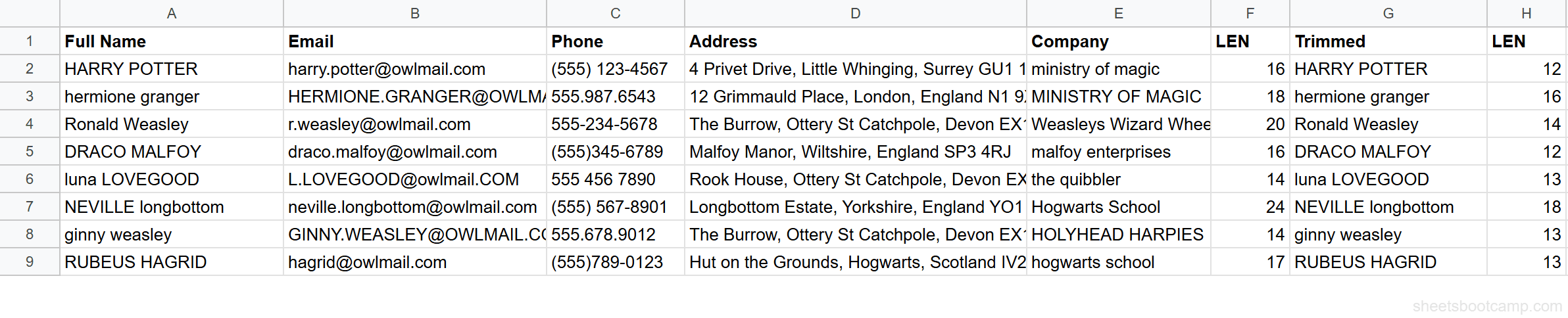
Verify with LEN
Use LEN to confirm TRIM worked. Enter =LEN(A2) and =LEN(TRIM(A2)) side by side:
| Name | LEN(A2) | LEN(TRIM(A2)) | Spaces Removed |
|---|---|---|---|
"HARRY POTTER" | 16 | 12 | 4 |
" Ronald Weasley " | 20 | 14 | 6 |
" NEVILLE longbottom " | 24 | 18 | 6 |
If both LEN values match, there were no extra spaces. If they differ, TRIM removed hidden whitespace.
Non-Breaking Spaces and CHAR(160)
TRIM handles regular spaces (CHAR(32)) but does not remove non-breaking spaces (CHAR(160)). Non-breaking spaces appear in data copied from web pages and word processors.
To remove them, use SUBSTITUTE to convert non-breaking spaces to regular spaces, then TRIM:
=TRIM(SUBSTITUTE(A2, CHAR(160), " "))This replaces every CHAR(160) with a regular space, then TRIM collapses the result. If your data still has spacing issues after TRIM, non-breaking spaces are the most likely cause.
Practical Examples
Example 1: Fix Broken VLOOKUP
A VLOOKUP returns #N/A even though the values look identical. The lookup column has trailing spaces.
=VLOOKUP(TRIM(A2), TRIM(B:B), 2, FALSE)TRIM both the lookup value and the lookup column. For even better protection, clean the source data once with TRIM and paste as values, so every formula using that column works correctly.
Example 2: Clean Before Comparing
You need to check if two names match. "HARRY POTTER" in cell A2 and "HARRY POTTER" in cell B2 look similar but are not equal.
=TRIM(A2)=TRIM(B2)This returns TRUE after TRIM normalizes both values. Without TRIM, the comparison returns FALSE because the space counts differ.
Example 3: Batch Clean with ARRAYFORMULA
To clean an entire column at once:
=ARRAYFORMULA(TRIM(CLEAN(A2:A9)))This applies TRIM and CLEAN to every cell in the range. Enter it in a helper column, then copy the results and paste over the originals with Paste special > Values only (Ctrl+Shift+V) to replace the messy data permanently.
Common Errors and How to Fix Them
TRIM Not Removing All Spaces
If spaces remain after TRIM, they are likely non-breaking spaces (CHAR(160)). Use =TRIM(SUBSTITUTE(A2, CHAR(160), " ")) to handle them.
LEN Still Shows Extra Characters After CLEAN
CLEAN removes characters 0-31 but not character 127 (DEL) or character 160 (non-breaking space). For a thorough cleanup, chain SUBSTITUTE calls for specific characters: =TRIM(CLEAN(SUBSTITUTE(A2, CHAR(160), " "))).
TRIM on Numbers Returns Text
=TRIM(12345) converts the number to a text string "12345". If you need the result as a number, wrap it in VALUE: =VALUE(TRIM(A2)). This matters when TRIM is part of a chain that feeds into numeric calculations.
Use =CODE(MID(A2, N, 1)) to check the ASCII code of a specific character in a string. Replace N with the character position. If the code is not 32 (regular space), you’ve found the hidden character causing problems.
Tips and Best Practices
-
TRIM imported data first, always. Extra spaces are the number one cause of broken VLOOKUP formulas and failed comparisons. TRIM the lookup columns before writing any formulas.
-
Use TRIM(CLEAN()) as your default cleanup pair. Even if the data looks clean, invisible characters can lurk. This two-function combo handles both categories of invisible problems.
-
Verify with LEN. If TRIM does not seem to fix the problem, compare
=LEN(A2)with=LEN(TRIM(A2)). If they are equal, the extra characters are not regular spaces — try SUBSTITUTE with CHAR(160). -
Paste as values after cleaning. Once your helper column has clean data, copy it and paste over the originals using Ctrl+Shift+V (Values only). This permanently replaces the messy data and removes the formula dependency.
-
Combine with case functions.
=TRIM(PROPER(A2))cleans spaces and fixes capitalization in one formula. This is the most common two-function combo for name cleanup.
Related Google Sheets Tutorials
- Text Functions in Google Sheets — Full guide to cleaning, extracting, and combining text data
- CONCATENATE and TEXTJOIN — Combine cleaned text from multiple cells
- SPLIT Function in Google Sheets — TRIM before splitting to avoid empty cells from extra spaces
- LEFT, RIGHT, MID — TRIM before extracting to get accurate character positions
- VLOOKUP in Google Sheets — TRIM lookup columns to fix #N/A errors from hidden spaces
Frequently Asked Questions
What does TRIM do in Google Sheets?
TRIM removes leading spaces, trailing spaces, and collapses multiple consecutive spaces between words down to a single space. =TRIM(" HARRY POTTER ") returns "HARRY POTTER" with one space between the words and no spaces at the start or end.
What is the difference between TRIM and CLEAN in Google Sheets?
TRIM removes extra spaces (leading, trailing, and repeated). CLEAN removes non-printable characters with ASCII codes 0 through 31, like line breaks, tabs, and control characters that sometimes appear in imported data. Use TRIM for space problems. Use CLEAN for invisible characters. For imported data, use both: =TRIM(CLEAN(A2)).
Why does my VLOOKUP fail even when the values look the same?
Extra spaces or invisible characters are the most common cause. The cell might contain " Harry" with a leading space, which does not match "Harry" in your lookup table. Apply =TRIM(A2) to both the lookup value and the lookup column to remove hidden spaces before running VLOOKUP.
How do I remove non-breaking spaces in Google Sheets?
TRIM does not remove non-breaking spaces (character 160). Use SUBSTITUTE to replace them: =SUBSTITUTE(A2, CHAR(160), " "). Then wrap it in TRIM: =TRIM(SUBSTITUTE(A2, CHAR(160), " ")). This converts non-breaking spaces to regular spaces, then TRIM collapses them.
Can I TRIM an entire column at once in Google Sheets?
Use ARRAYFORMULA with TRIM. Enter =ARRAYFORMULA(TRIM(A2:A100)) in a helper column. This applies TRIM to every cell in the range. To replace the original values, copy the helper column, then paste over the original with Paste special > Values only (Ctrl+Shift+V).