VLOOKUP from Another Sheet in Google Sheets
Pull data from another sheet or tab using VLOOKUP in Google Sheets. Step-by-step guide covering sheet reference syntax, naming rules, and real examples.
Sheets Bootcamp
February 22, 2026
VLOOKUP in Google Sheets can pull data from another sheet in the same spreadsheet. You add the tab name and an exclamation mark to the range reference, and VLOOKUP searches that sheet instead of the current one. This is how most real workbooks are set up: a lookup table on one tab, data entry on another.
This article covers the sheet reference syntax, a step-by-step example using product inventory data, and how to handle sheet names with spaces.
How Sheet References Work
When you write a VLOOKUP formula, the range parameter normally points to cells on the current sheet. To reference a different tab, add the sheet name followed by an exclamation mark before the range.
=VLOOKUP(A2, Products!A2:D6, 4, FALSE)In this formula, Products!A2:D6 tells Google Sheets to look at cells A2 through D6 on the tab named Products. The exclamation mark separates the sheet name from the cell range.
If the sheet name contains spaces, special characters, or starts with a number, wrap it in single quotes:
=VLOOKUP(A2, 'Product List'!A2:D6, 4, FALSE)Without the quotes, Google Sheets returns a formula parse error.
You do not need to type the sheet reference manually. While writing a formula, click on the other tab and select the range. Google Sheets adds the sheet name and exclamation mark for you.
VLOOKUP from Another Tab: Step-by-Step
Here is a complete walkthrough. You have a product inventory on the Products tab and need to pull prices into an Orders tab.
Set up your lookup table on the Products sheet
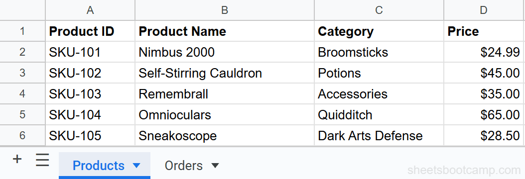
The Products sheet holds your inventory data in columns A through D:
| A | B | C | D | |
|---|---|---|---|---|
| 1 | Product ID | Product Name | Category | Price |
| 2 | SKU-101 | Nimbus 2000 | Broomsticks | $24.99 |
| 3 | SKU-102 | Self-Stirring Cauldron | Potions | $45.00 |
| 4 | SKU-103 | Remembrall | Accessories | $35.00 |
| 5 | SKU-104 | Omnioculars | Quidditch | $65.00 |
| 6 | SKU-105 | Sneakoscope | Dark Arts Defense | $28.50 |
Product ID is in the first column. This is required because VLOOKUP always searches the leftmost column of the range.
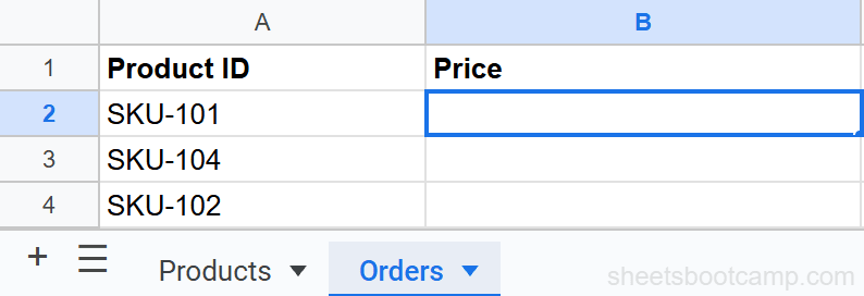
Switch to the Orders sheet
The Orders sheet is where you enter order data. Column A has the Product ID for each order. Column B is where the price will go.
| A | B | |
|---|---|---|
| 1 | Product ID | Price |
| 2 | SKU-101 | |
| 3 | SKU-104 | |
| 4 | SKU-102 |
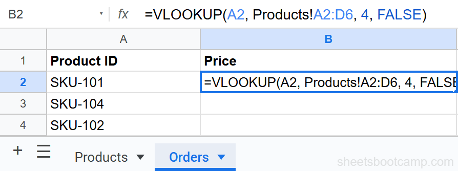
Write the VLOOKUP formula with a sheet reference
Select cell B2 on the Orders sheet and enter:
=VLOOKUP(A2, Products!A2:D6, 4, FALSE)Here is what each part does:
A2— the Product ID on the Orders sheet (SKU-101)Products!A2:D6— the range on the Products tab to search4— return the value from the 4th column (Price)FALSE— find an exact match
The Products! prefix is the only difference from a regular VLOOKUP. Everything else works the same way.
You can also write the formula by typing =VLOOKUP(A2, and then clicking the Products tab. Select the range A2:D6, and Google Sheets inserts Products!A2:D6 for you. Press Enter to finish.
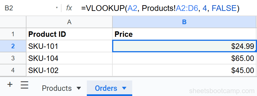
Check the result
The formula returns $24.99, the price for SKU-101, pulled from the Products sheet. Copy the formula down to B3 and B4 to look up the remaining products. SKU-104 returns $65.00 and SKU-102 returns $45.00.
Sheet Names with Spaces
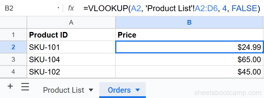
If your tab is named Product List instead of Products, you need single quotes around the sheet name:
=VLOOKUP(A2, 'Product List'!A2:D6, 4, FALSE)Single quotes are required when the sheet name contains:
- Spaces —
'Product List'!A2:D6 - Special characters —
'Q1-2026 Data'!A2:D6 - A leading number —
'2026 Sales'!A2:D6
Forgetting the single quotes around a sheet name with spaces causes a formula parse error. If you click on the other tab while writing the formula, Google Sheets adds the quotes automatically.
VLOOKUP from a Different Spreadsheet
Sheet references only work within the same spreadsheet file. The Products!A2:D6 syntax references a tab, not an external file.
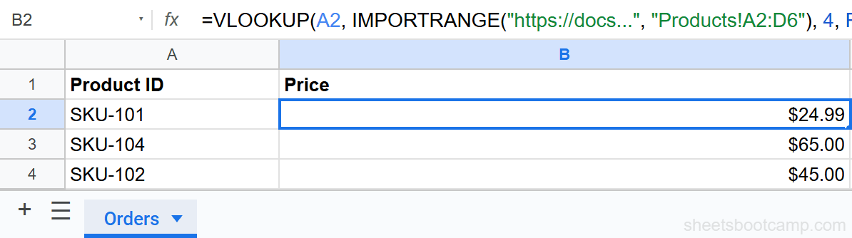
To pull data from a completely different Google Sheets file, combine VLOOKUP with IMPORTRANGE:
=VLOOKUP(A2, IMPORTRANGE("spreadsheet_url", "Products!A2:D6"), 4, FALSE)Replace spreadsheet_url with the full URL of the other spreadsheet. The first time you use IMPORTRANGE with a new file, Google Sheets asks you to grant access. Click Allow access when prompted.
IMPORTRANGE has a performance cost. If you are pulling large ranges from external spreadsheets, your formulas may take several seconds to calculate. See the IMPORTRANGE guide for optimization tips.
Common Errors
#REF! Error
The sheet name is misspelled or the tab was deleted. Double-check that the tab name in your formula matches exactly, including capitalization. If you renamed the sheet, Google Sheets usually updates references automatically. But if you typed the reference manually, you need to update it yourself.
#N/A Error
The lookup value was not found on the other sheet. This works the same as a regular VLOOKUP error. Check for extra spaces, typos, or mismatched data types between the two sheets.
Formula Parse Error
The sheet name contains spaces but is missing single quotes. Change Product List!A2:D6 to 'Product List'!A2:D6.
Tips for Cross-Sheet VLOOKUP
-
Use absolute references when copying formulas down. Change
Products!A2:D6toProducts!$A$2:$D$6so the range stays fixed when you drag the formula to other rows. -
Let Google Sheets auto-complete the reference. Click on the other tab while writing the formula instead of typing the sheet name manually. This avoids typos and adds quotes when needed.
-
Name your sheets clearly. Use descriptive tab names like “Products” or “Employees” instead of “Sheet1” or “Sheet2.” Your formulas become easier to read and maintain.
-
Avoid spaces in sheet names when possible. Names like
ProductsandOrdersdo not need single quotes. Names likeProduct Listrequire extra syntax.
If multiple formulas reference the same sheet, consider using a named range. Go to Data > Named ranges and give your lookup table a name like ProductTable. Then use =VLOOKUP(A2, ProductTable, 4, FALSE) with no sheet reference needed.
Related Google Sheets Tutorials
- VLOOKUP: The Complete Guide - Full VLOOKUP syntax, examples, and best practices
- VLOOKUP for Beginners - Start here if VLOOKUP is new to you
- Fix VLOOKUP Errors - Troubleshoot #N/A, #REF!, and #VALUE! errors
- IMPORTRANGE in Google Sheets - Pull data from a different spreadsheet file
- INDEX MATCH in Google Sheets - A more flexible alternative to VLOOKUP
Frequently Asked Questions
Can VLOOKUP pull data from another sheet?
Yes. Add the sheet name and an exclamation mark before the range reference. For example, =VLOOKUP(A2, Products!A2:D6, 4, FALSE) searches the Products sheet.
How do I reference a sheet name with spaces?
Wrap the sheet name in single quotes. For example, 'Product List'!A2:D6. Without the quotes, Google Sheets returns a formula parse error.
Can VLOOKUP pull data from a different spreadsheet?
Not directly. VLOOKUP works across sheets (tabs) within the same spreadsheet. To pull from a different spreadsheet file, combine VLOOKUP with IMPORTRANGE.
What happens if I rename the sheet?
Google Sheets updates sheet references automatically when you rename a tab. Your VLOOKUP formulas continue working without any changes.
Why does my cross-sheet VLOOKUP show #REF!?
The #REF! error usually means the sheet name is misspelled or the sheet was deleted. Double-check the tab name matches exactly, including capitalization.