VLOOKUP for Beginners in Google Sheets
Learn VLOOKUP in Google Sheets from scratch with this step-by-step beginner tutorial. Covers syntax, real examples, common mistakes, and practical tips.
Sheets Bootcamp
February 19, 2026
VLOOKUP for beginners starts with one idea: you have a value, and you want to find related data in a table. VLOOKUP in Google Sheets searches down the first column of a range and returns a value from any column in that same row. This guide walks you through your first VLOOKUP formula, explains every parameter, and covers the mistakes most beginners run into.
What Is VLOOKUP?
VLOOKUP stands for Vertical Lookup. It scans down the first column of a range looking for a match, then returns a value from a column you specify.
Think of it like a contacts list on your phone. You search for a person’s name (the lookup value), and your phone returns their number (the value from another column). VLOOKUP works the same way, except the “contacts list” is a range of cells in your spreadsheet, and you choose which column of information to pull back.
VLOOKUP has opinions about column order. Your lookup value must be in the first column of the range, no exceptions.
VLOOKUP Syntax
Here is the VLOOKUP formula structure in Google Sheets:
=VLOOKUP(search_key, range, index, [is_sorted])| Parameter | Description | Required |
|---|---|---|
| search_key | The value you want to find in the first column of your range | Yes |
| range | The block of cells containing your data (lookup table) | Yes |
| index | The column number within the range to return a value from. Column 1 is the first column of the range, not the sheet. | Yes |
| is_sorted | FALSE for exact match, TRUE for approximate match. Defaults to TRUE if omitted. | No |
The search_key must exist in the first (leftmost) column of your range. VLOOKUP only searches that column. If your data is arranged differently, use INDEX MATCH instead.
How to Use VLOOKUP: Step-by-Step
We’ll use a product inventory with 5 items. The goal: look up the price for a specific product ID.
Set up your data
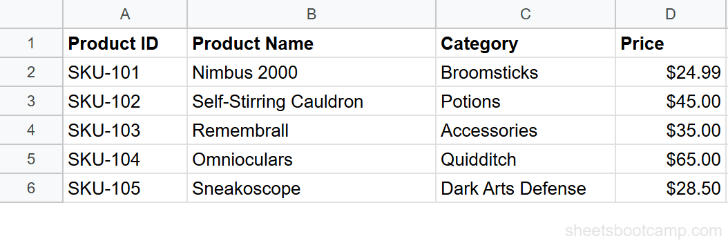
Your spreadsheet has a product inventory in columns A through F. Each row contains a Product ID, Product Name, Category, Price, Stock count, and Supplier.
| A | B | C | D | E | F | |
|---|---|---|---|---|---|---|
| 1 | Product ID | Product Name | Category | Price | Stock | Supplier |
| 2 | SKU-101 | Nimbus 2000 | Broomsticks | $24.99 | 150 | Quality Quidditch Supplies |
| 3 | SKU-102 | Self-Stirring Cauldron | Potions | $45.00 | 75 | Weasleys Wizard Wheezes |
| 4 | SKU-103 | Remembrall | Accessories | $35.00 | 200 | Dervish and Banges |
| 5 | SKU-104 | Omnioculars | Quidditch | $65.00 | 50 | Quality Quidditch Supplies |
| 6 | SKU-105 | Sneakoscope | Dark Arts Defense | $28.50 | 120 | Dervish and Banges |
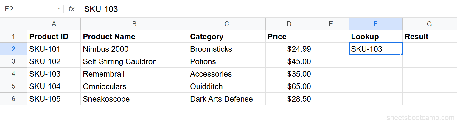
Decide what to look up
You want to find the price for SKU-103. Enter SKU-103 in cell F2 as your lookup value. You will write the VLOOKUP formula in cell G2 to return the matching price.
Write the formula
Select cell G2 and enter this formula:
=VLOOKUP("SKU-103", A2:D6, 4, FALSE)Here is what each part does:
"SKU-103"— the Product ID you are searching forA2:D6— the range containing your data (Product ID through Price)4— return the value from the 4th column in the range. Column A (Product ID) is 1, Column B (Product Name) is 2, Column C (Category) is 3, and Column D (Price) is 4.FALSE— match the search key exactly
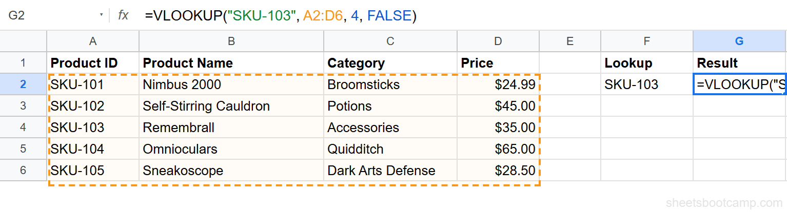
The index counts columns within your range, not columns on the sheet. Price is in column D on the sheet, but it is the 4th column in the range A2:D6. That is why the index is 4.
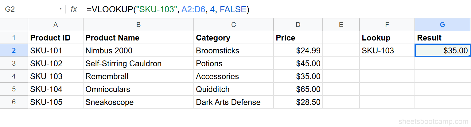
Check the result
Press Enter. The formula returns $35.00, the price for the Remembrall (SKU-103).
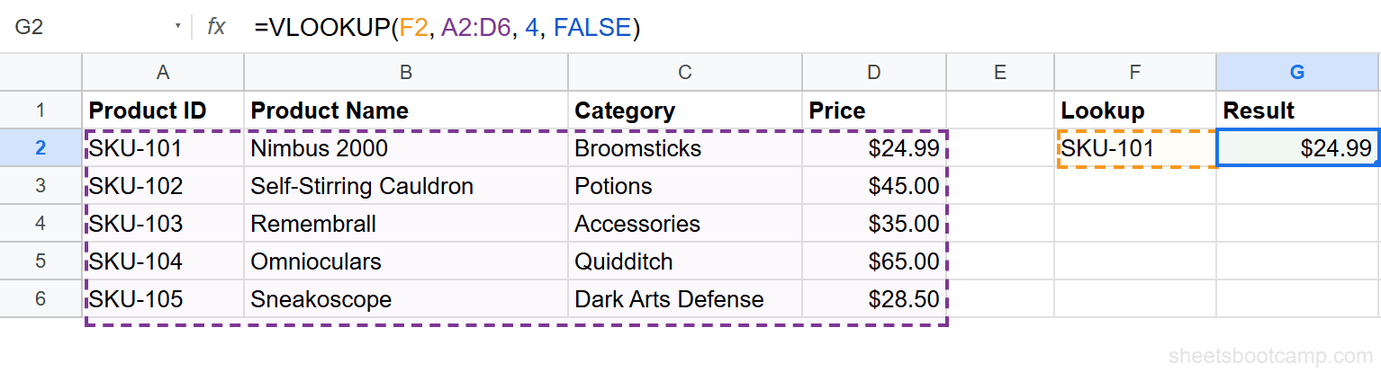
Make VLOOKUP Dynamic with Cell References
Hardcoding "SKU-103" in the formula works, but it means you have to edit the formula every time you want to look up a different product. A better approach: reference a cell.
Enter any Product ID in cell F2, then change the formula to:
=VLOOKUP(F2, A2:D6, 4, FALSE)Now the formula reads the search key from F2. Type SKU-101 in F2, and G2 updates to $24.99. Type SKU-104, and it returns $65.00. You change the input, and the output follows.
This is how VLOOKUP is used in practice. You rarely hardcode the search key.
Common Beginner Mistakes
Wrong column index
The index counts columns within your range, not from column A of the sheet. If your range is A2:D6, column A is 1, column B is 2, column C is 3, and column D is 4. Using 4 when your range only has 3 columns triggers a #REF! error.
Count from the first column of your range, not the first column of the sheet.
Forgetting FALSE
VLOOKUP defaults to approximate match (TRUE) when you leave out the fourth parameter. Approximate match requires sorted data and can return wrong values without any warning.
Omitting the last parameter or setting it to TRUE on unsorted data returns incorrect results silently. You will not see an error. Always include FALSE for exact matching.
Search key not in first column
VLOOKUP searches the first column of your range only. If you set the range to B2:D6, VLOOKUP searches column B. If your Product IDs are in column A but your range starts at column B, the formula will search Product Names instead and likely return #N/A.
Make sure your range starts at the column containing the value you want to match.
Tips for Beginners
1. Always use FALSE for exact match. Approximate match is a special case. For everyday lookups, FALSE is the correct choice.
2. Lock your range with $ signs. If you plan to copy the formula to other rows, use $A$2:$D$6 instead of A2:D6. The dollar signs prevent the range from shifting when you copy down.
3. Wrap in IFERROR for cleaner results. When the search key is not found, VLOOKUP shows #N/A. You can return a custom message instead:
Use =IFERROR(VLOOKUP(F2, $A$2:$D$6, 4, FALSE), "Not found") to display “Not found” instead of #N/A. This keeps your sheet readable when lookup values are missing.
Related Google Sheets Tutorials
- VLOOKUP: The Complete Guide — covers syntax, approximate match, and alternatives
- Fix VLOOKUP Errors — troubleshoot #N/A, #REF!, and #VALUE! errors
- VLOOKUP from Another Sheet — pull data from a different tab
- INDEX MATCH in Google Sheets — a more flexible alternative to VLOOKUP
Frequently Asked Questions
What does VLOOKUP stand for?
VLOOKUP stands for Vertical Lookup. It searches vertically down the first column of a range to find a matching value, then returns data from a specified column in that same row.
Is VLOOKUP hard to learn?
VLOOKUP has four parameters, but it follows a consistent pattern. Once you understand what each parameter does, you can apply the same structure to any lookup. Most beginners pick it up in under 30 minutes.
Can VLOOKUP search left?
No. VLOOKUP only searches the first (leftmost) column of your range and returns values from columns to the right. If you need to look left, use INDEX MATCH instead.
What is the difference between TRUE and FALSE in VLOOKUP?
FALSE finds an exact match. TRUE finds an approximate match, returning the closest value less than or equal to your search key. Use FALSE in most cases — TRUE requires sorted data and can return wrong results silently.
Why does my VLOOKUP return #N/A?
The #N/A error means VLOOKUP could not find your search key in the first column of the range. Common causes include typos, extra spaces, or mismatched data types. Use TRIM to clean data and double-check spelling.