Fix VLOOKUP Errors in Google Sheets
Fix VLOOKUP errors in Google Sheets including #N/A, #REF!, #VALUE!, and wrong results. Find the cause of each error and resolve it with formula examples.
Sheets Bootcamp
February 20, 2026
VLOOKUP errors in Google Sheets usually come down to a handful of causes, and most have a quick fix once you know where to look. If your VLOOKUP formula is returning #N/A, #REF!, or #VALUE!, this guide will help you identify the problem and resolve it. We also cover the trickier case where VLOOKUP returns a result but the value is wrong.
In This Guide
- Sample Data
- #N/A Error
- #REF! Error
- #VALUE! Error
- VLOOKUP Returns the Wrong Value
- How to Prevent VLOOKUP Errors
- Related Google Sheets Tutorials
- FAQ
Sample Data
We’ll use this product inventory table for every example in this guide. The data lives in columns A through D with five products.
| Product ID | Product Name | Category | Price |
|---|---|---|---|
| SKU-101 | Nimbus 2000 | Broomsticks | $24.99 |
| SKU-102 | Self-Stirring Cauldron | Potions | $45.00 |
| SKU-103 | Remembrall | Accessories | $35.00 |
| SKU-104 | Omnioculars | Quidditch | $65.00 |
| SKU-105 | Sneakoscope | Dark Arts Defense | $28.50 |
#N/A Error
The #N/A error is the most common VLOOKUP error. It means the search key was not found in the first column of your range. There are several reasons this happens.
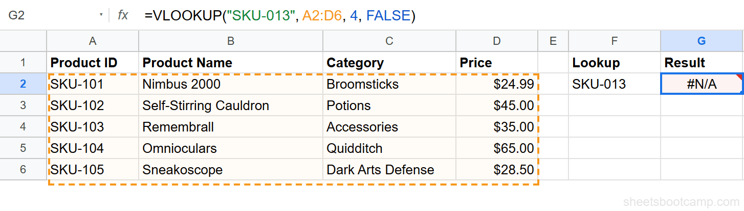
Cause 1: Typos or Misspellings
If you search for "SKU-013" instead of "SKU-103", VLOOKUP cannot find a match and returns #N/A. Double-check the spelling of your search key against the actual data.
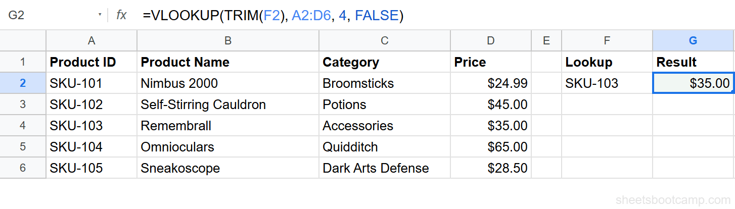
Cause 2: Extra Spaces
A cell that looks like it contains SKU-103 might actually contain " SKU-103" or "SKU-103 ". The space is invisible but enough to prevent a match.
Use TRIM to remove leading and trailing spaces from both sides of the lookup:
=VLOOKUP(TRIM(F2), A2:D6, 4, FALSE)This strips whitespace from the search key in F2 before VLOOKUP runs. If the extra spaces are in your lookup column, clean that column with TRIM as well.
Cause 3: Number Stored as Text
Your Product ID column might contain "103" stored as text, but the search key is the number 103. Google Sheets treats these as different values.
To fix this, convert the search key to match the data type. If your lookup column has text values, wrap the search key in TEXT: =VLOOKUP(TEXT(F2, "0"), A2:D6, 4, FALSE). If the lookup column has numbers, use VALUE: =VLOOKUP(VALUE(F2), A2:D6, 4, FALSE).
Cause 4: Search Key Not in the First Column
VLOOKUP only searches the first column of your range. If you set the range to B2:D6, VLOOKUP searches column B (Product Name), not column A (Product ID). If your search key is a Product ID, the range must start at column A.
Fix: adjust your range so the column containing the search key is the first column. If your data layout does not allow this, use INDEX MATCH instead.
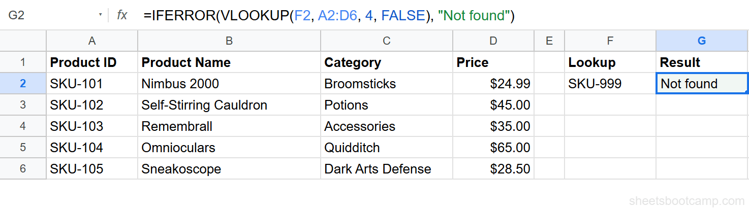
Wrap VLOOKUP in IFERROR to return a custom message instead of #N/A. For example, =IFERROR(VLOOKUP(F2, A2:D6, 4, FALSE), "Not found") keeps your sheet readable when a lookup value is missing.
#REF! Error
The #REF! error means the reference is invalid. In VLOOKUP, this almost always involves the column index number.
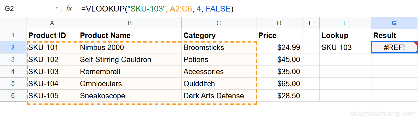
Cause 1: Column Index Exceeds Range Width
If your range is A2:C6, you have 3 columns: A (column 1), B (column 2), and C (column 3). Setting the column index to 4 asks VLOOKUP for a fourth column that does not exist. Google Sheets returns #REF!.
=VLOOKUP("SKU-103", A2:C6, 4, FALSE)This formula breaks because A2:C6 has only 3 columns.
Fix: count the columns in your range, starting from the first column of the range. If you need data from column D, extend the range to A2:D6 and set the index to 4.
Count columns from the start of your range, not from column A of the sheet. If your range starts at C2, then C is column 1, D is column 2, and so on.
Cause 2: Invalid Sheet Reference
If your VLOOKUP references another sheet and that sheet has been deleted or renamed, Google Sheets returns #REF!.
Fix: check the sheet name in your formula. Open the formula bar, look for the sheet reference (e.g., 'Inventory'!A2:D6), and confirm the sheet name matches exactly, including any spaces or special characters.
#VALUE! Error
The #VALUE! error means one of the arguments is the wrong type. This error is less common than #N/A or #REF!, but it still shows up.
Cause 1: Column Index Is Not a Number
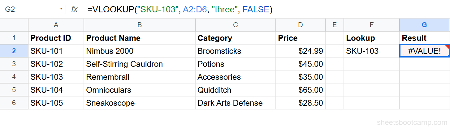
If you accidentally pass text as the third argument, VLOOKUP returns #VALUE!. For example:
=VLOOKUP("SKU-103", A2:D6, "three", FALSE)The string "three" is not a valid column index. The third argument must be a number.
Fix: replace the text with a number. In this case, use 3 instead of "three".
Cause 2: Invalid Range Syntax
A typo in the range can trigger #VALUE!. For example, A2:D (missing the row number) or A2D6 (missing the colon) are not valid ranges.
Fix: correct the range syntax. A valid range looks like A2:D6 or A:D.
VLOOKUP Returns the Wrong Value
This is not an error message. The formula runs, returns a value, and looks normal. But the result is wrong. This is the most dangerous scenario because nothing signals that the output is incorrect.
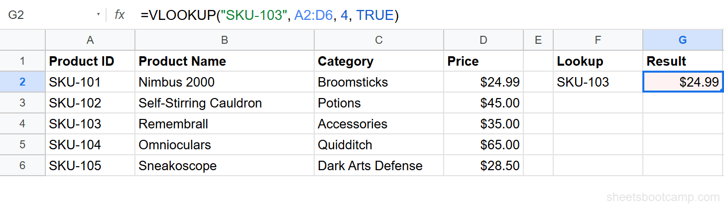
Cause 1: Using TRUE on Unsorted Data
When the fourth argument is TRUE (or omitted, since TRUE is the default), VLOOKUP performs a binary search. Binary search assumes the first column is sorted in ascending order. If the data is not sorted, VLOOKUP picks the wrong row.
=VLOOKUP("SKU-103", A2:D6, 4, TRUE)On unsorted data, this might return $24.99 instead of $35.00, and Google Sheets will not warn you.
Fix: change TRUE to FALSE. Use FALSE for exact matching in almost every case.
Using TRUE (approximate match) on unsorted data returns wrong results without any error message. You will not know the output is incorrect. Always use FALSE unless your first column is sorted in ascending order and you specifically need range-based matching.
Cause 2: Wrong Column Index
If you count columns from column A of the sheet instead of from the start of your range, you might pull data from the wrong column.
For example, if your range is B2:D6, then B is column 1, C is column 2, and D is column 3. Setting the index to 3 returns column D, not column C.
Fix: always count from the first column of the range.
Cause 3: Duplicate Values in the Lookup Column
VLOOKUP returns the first match it finds. If the lookup column contains duplicate values, VLOOKUP always returns data from the first matching row, even if a different row is the one you need.
Fix: remove duplicates from the lookup column, or switch to a unique identifier like Product ID. If you need to look up based on multiple conditions, use VLOOKUP with multiple criteria.
How to Prevent VLOOKUP Errors
A few habits prevent most VLOOKUP errors before they happen.
Wrap in IFERROR. IFERROR catches any error and returns a value you choose. This keeps your sheet clean and readable.
=IFERROR(VLOOKUP(F2, A2:D6, 4, FALSE), "Not found")If VLOOKUP cannot find the search key, the cell shows “Not found” instead of #N/A.
Clean your data with TRIM. Extra spaces are invisible and cause more #N/A errors than almost anything else. Run =TRIM() on both the search key and the lookup column.
Always use FALSE. Unless you specifically need approximate matching on sorted data, set the fourth argument to FALSE. This ensures exact matching and eliminates silent wrong results.
Use data validation on input cells. If users enter search keys manually, restrict the input to valid values. A dropdown list built from the lookup column prevents typos and mismatches.
IFERROR catches all errors, not only #N/A. If your formula has a #REF! error from a bad column index, IFERROR will hide it. Fix the root cause first, then add IFERROR as a safety net.
Related Google Sheets Tutorials
- VLOOKUP in Google Sheets: Complete Guide - Full syntax breakdown, step-by-step examples, and best practices
- VLOOKUP for Beginners - Start here if you are new to VLOOKUP
- VLOOKUP with Multiple Criteria - Look up values using more than one condition
- VLOOKUP from Another Sheet - Pull data across sheets and spreadsheets
- INDEX MATCH in Google Sheets - A more flexible alternative that avoids several VLOOKUP limitations
FAQ
Why does VLOOKUP return #N/A?
The #N/A error means VLOOKUP could not find the search key in the first column of the range. Common causes include typos, extra spaces, number-vs-text mismatches, and the search key not being in the first column.
How do I fix #REF! in VLOOKUP?
The #REF! error means the column index number is larger than the number of columns in your range. Count the columns in your range and make sure the index number does not exceed that count.
Why does VLOOKUP return the wrong value?
If VLOOKUP returns a value but it is incorrect, the most common cause is using TRUE (approximate match) on unsorted data. Change the last parameter to FALSE for exact matching.
What does IFERROR do with VLOOKUP?
IFERROR wraps around VLOOKUP and returns a custom value when VLOOKUP produces an error. For example, =IFERROR(VLOOKUP(A2, range, 2, FALSE), “Not found”) shows “Not found” instead of #N/A.
Can extra spaces cause VLOOKUP errors?
Yes. Leading or trailing spaces make values look identical but not match. Use =TRIM() on both the search key and the lookup column to remove extra spaces before running VLOOKUP.