VLOOKUP Multiple Criteria in Google Sheets
Learn how to use VLOOKUP with multiple criteria in Google Sheets. Two proven methods with step-by-step examples: helper column and ARRAYFORMULA approach.
Sheets Bootcamp
February 21, 2026
VLOOKUP with multiple criteria in Google Sheets requires a workaround because VLOOKUP only searches one column. When your data has duplicate values that need a second condition to tell apart, a standard VLOOKUP returns the first match and ignores the rest.
This article covers two methods to solve the problem: a helper column approach and an ARRAYFORMULA approach that skips the extra column entirely.
In This Guide
- The Problem: One Search Column Is Not Enough
- Method 1: Helper Column
- Method 2: ARRAYFORMULA (No Helper Column)
- When to Use INDEX MATCH Instead
- Tips and Best Practices
- Related Google Sheets Tutorials
- Frequently Asked Questions
The Problem: One Search Column Is Not Enough
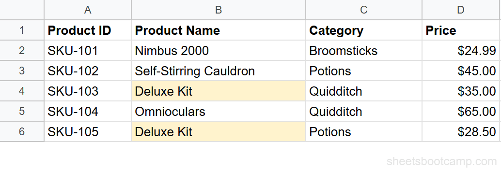
Consider this product inventory:
| Product ID | Product Name | Category | Price |
|---|---|---|---|
| SKU-101 | Nimbus 2000 | Broomsticks | $24.99 |
| SKU-102 | Self-Stirring Cauldron | Potions | $45.00 |
| SKU-103 | Deluxe Kit | Quidditch | $35.00 |
| SKU-104 | Omnioculars | Quidditch | $65.00 |
| SKU-105 | Deluxe Kit | Potions | $28.50 |
“Deluxe Kit” appears twice: once under Quidditch ($35.00) and once under Potions ($28.50). A standard VLOOKUP on Product Name returns the first match it finds.
=VLOOKUP("Deluxe Kit", B2:D6, 3, FALSE)This returns $35.00 (the Quidditch row) even if you wanted the Potions price. VLOOKUP stops at the first match and has no way to check a second condition.
You need to match on both Product Name and Category. VLOOKUP cannot do this on its own, but two workarounds make it possible.
Method 1: Helper Column
The helper column approach creates a new column that combines your criteria into a single searchable value. VLOOKUP then searches that combined column instead.
Add a helper column that combines your criteria
In cell E2, enter a formula that concatenates Category and Product Name with a separator:
=C2&"-"&B2This produces Quidditch-Deluxe Kit for row 2. The separator prevents false matches. Without it, “Potions” + “Kit” and “Potion” + “sKit” would produce the same string.
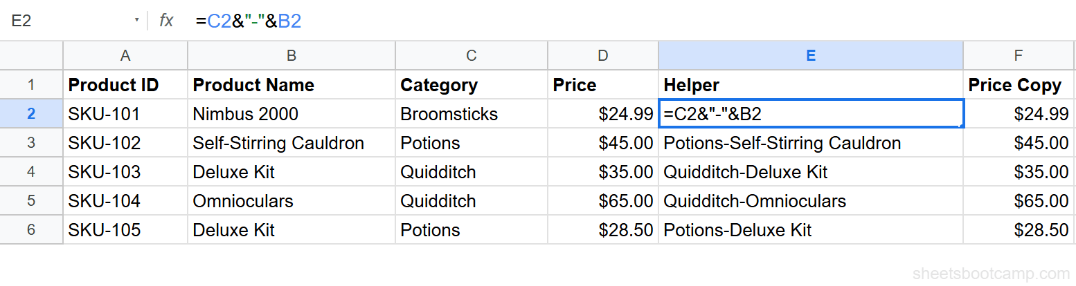
Add a return value column next to the helper
VLOOKUP returns values from columns to the right of the search column. Since Price (column D) is to the left of the helper (column E), you need a copy of Price to the right.
In cell F2, enter:
=D2This places the Price value next to the helper column where VLOOKUP can reach it.
Fill both columns down
Select E2:F2 and drag the fill handle down through row 6. Your helper column now contains:
| E (Helper) | F (Price) |
|---|---|
| Broomsticks-Nimbus 2000 | $24.99 |
| Potions-Self-Stirring Cauldron | $45.00 |
| Quidditch-Deluxe Kit | $35.00 |
| Quidditch-Omnioculars | $65.00 |
| Potions-Deluxe Kit | $28.50 |
Write the VLOOKUP formula
Now use VLOOKUP to search the helper column. To find the price of the Potions Deluxe Kit:
=VLOOKUP("Potions-Deluxe Kit", E2:F6, 2, FALSE)This returns $28.50. The formula searches column E for the exact string “Potions-Deluxe Kit” and returns the value from column F.
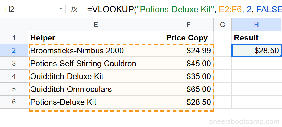
To make this dynamic, reference cells instead of hardcoding:
=VLOOKUP(H2&"-"&G2, E2:F6, 2, FALSE)Where H2 contains the category and G2 contains the product name.
Use a separator like "-" or "|" in your concatenation. Without one, "AB"&"CD" and "A"&"BCD" both produce "ABCD", which causes false matches.
Method 2: ARRAYFORMULA (No Helper Column)
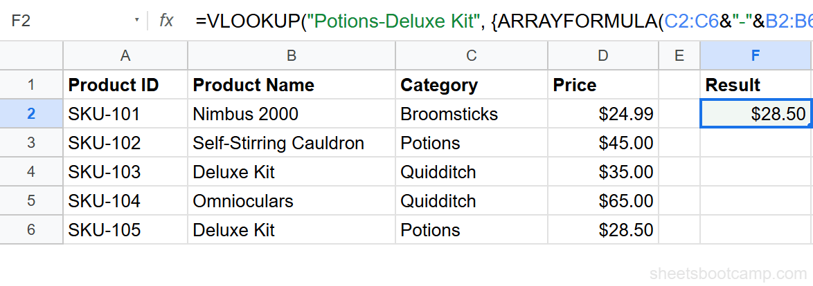
The ARRAYFORMULA method builds the helper column on the fly inside the formula. No extra columns needed.
=VLOOKUP("Potions-Deluxe Kit", {ARRAYFORMULA(C2:C6&"-"&B2:B6), D2:D6}, 2, FALSE)Here is how it works:
ARRAYFORMULA(C2:C6&"-"&B2:B6)creates a virtual column of concatenated values (the same as the helper column from Method 1)D2:D6is the Price column you want to return- The curly braces
{ }join these two arrays into a temporary two-column range - VLOOKUP searches the first column of that range and returns from the second
This returns $28.50, the same result as the helper column method.
To make the search key dynamic:
=VLOOKUP(H2&"-"&G2, {ARRAYFORMULA(C2:C6&"-"&B2:B6), D2:D6}, 2, FALSE)Array formulas with curly braces are harder to debug when something goes wrong. If you are new to VLOOKUP, start with the helper column method. Move to ARRAYFORMULA once you are comfortable with the logic.
When to Use INDEX MATCH Instead
INDEX MATCH handles multiple criteria without helper columns or array syntax. It uses a different approach: multiply conditions together inside MATCH to create an array filter.
=INDEX(D2:D6, MATCH(1, (B2:B6="Deluxe Kit")*(C2:C6="Potions"), 0))This formula checks both conditions at once and returns $28.50. No concatenation, no curly braces, no extra columns.
The tradeoff is syntax. INDEX MATCH with multiple criteria requires pressing Ctrl+Shift+Enter in some spreadsheet apps (though Google Sheets handles it automatically). The formula is also longer to read.
For one-off lookups, either VLOOKUP method in this article works well. For recurring multi-criteria lookups across large datasets, INDEX MATCH is the more maintainable choice.
The QUERY function is another alternative. It handles multiple WHERE conditions and is often more readable for filtering tasks.
Google Sheets evaluates the INDEX MATCH array formula automatically. You do not need Ctrl+Shift+Enter like in Excel.
Tips and Best Practices
-
Use a consistent separator. Pick one character (
-,|, or~) and use it across all helper columns in your workbook. This makes formulas predictable. -
Hide the helper columns. Right-click the column header and select “Hide column” to keep your sheet clean while preserving the lookup functionality.
-
Test with a known value first. Before building a dynamic formula, hardcode the search key to confirm the lookup works. Then swap in cell references.
-
Watch for extra spaces. If your concatenated key does not match, wrap the source values in
TRIM():=TRIM(C2)&"-"&TRIM(B2). Trailing spaces are invisible but break exact matches. -
Consider INDEX MATCH for ongoing use. If you find yourself adding helper columns to multiple sheets, switching to INDEX MATCH saves time and keeps your data cleaner.
Related Google Sheets Tutorials
- VLOOKUP in Google Sheets: Complete Guide - Full syntax breakdown, examples, and error handling for standard VLOOKUP
- INDEX MATCH in Google Sheets - A more flexible lookup method that handles left lookups and multiple criteria natively
- QUERY Function in Google Sheets - Filter and summarize data with SQL-like syntax, including multi-condition WHERE clauses
- Fix Common VLOOKUP Errors - Troubleshoot #N/A, #REF!, and #VALUE! errors in your VLOOKUP formulas
- VLOOKUP for Beginners - Start here if you need a refresher on basic VLOOKUP before adding multiple criteria
Frequently Asked Questions
Can VLOOKUP handle multiple criteria?
Not directly. VLOOKUP searches one column only. To match on multiple criteria, use a helper column that concatenates the criteria, or use an ARRAYFORMULA-based approach.
What is a helper column in Google Sheets?
A helper column is an extra column you add to your data that combines values from other columns. For multi-criteria VLOOKUP, you concatenate the criteria values so VLOOKUP can match on the combined string.
Is INDEX MATCH better for multiple criteria lookups?
Yes. INDEX MATCH handles multiple criteria natively using array formulas without needing a helper column. It is cleaner for complex lookups, though the syntax takes more practice.
Does the helper column order matter?
Yes. The concatenation order in your helper column must match the order in your search key. If the helper column combines Category and Product Name, your lookup value must concatenate them in the same order.
Can I use QUERY instead of VLOOKUP for multiple criteria?
Yes. The QUERY function handles multiple conditions with WHERE clauses. For complex multi-criteria lookups, QUERY is often more readable than VLOOKUP workarounds.