XLOOKUP in Google Sheets: Complete Guide
Learn how to use XLOOKUP in Google Sheets with step-by-step examples. Covers syntax, reverse lookups, wildcards, approximate match, and VLOOKUP comparison.
Sheets Bootcamp
March 26, 2026
XLOOKUP is a lookup function in Google Sheets that searches a range for a value and returns a result from a corresponding range. It replaces VLOOKUP in most situations — and fixes several of its biggest limitations. XLOOKUP can search in any direction, defaults to exact match, and has built-in error handling.
This guide covers the full XLOOKUP syntax, step-by-step examples, reverse lookups, wildcards, approximate matching, and a direct comparison with both VLOOKUP and INDEX MATCH.
XLOOKUP Syntax
Here is the full XLOOKUP syntax in Google Sheets:
=XLOOKUP(search_key, lookup_range, result_range, [missing_value], [match_mode], [search_mode])| Parameter | Required | Description |
|---|---|---|
| search_key | Yes | The value to search for |
| lookup_range | Yes | A single row or column to search in |
| result_range | Yes | The row or column to return values from (must match the size of lookup_range) |
| missing_value | No | Value to return if no match is found (defaults to #N/A) |
| match_mode | No | 0 = exact (default), 1 = next larger, -1 = next smaller, 2 = wildcard |
| search_mode | No | 1 = first to last (default), -1 = last to first, 2 = binary ascending, -2 = binary descending |
XLOOKUP defaults to exact match (match_mode 0). Unlike VLOOKUP, you do not need to add FALSE at the end of every formula.
The first three parameters handle most lookups. The last three are optional and cover edge cases like partial matching, error messages, and searching large sorted datasets.
How to Use XLOOKUP (Step-by-Step)
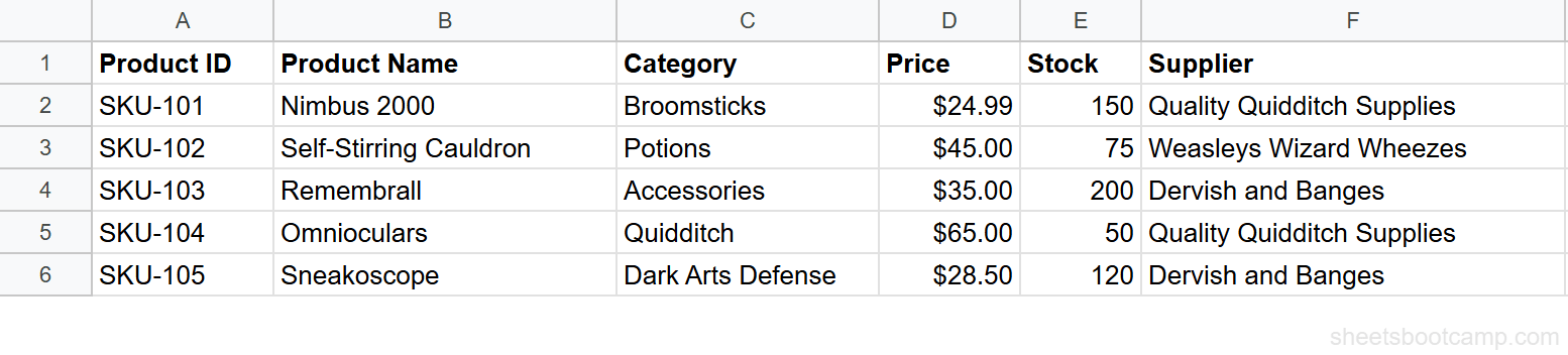
Here is a product inventory table. The goal is to look up a Product ID and return the matching Product Name.
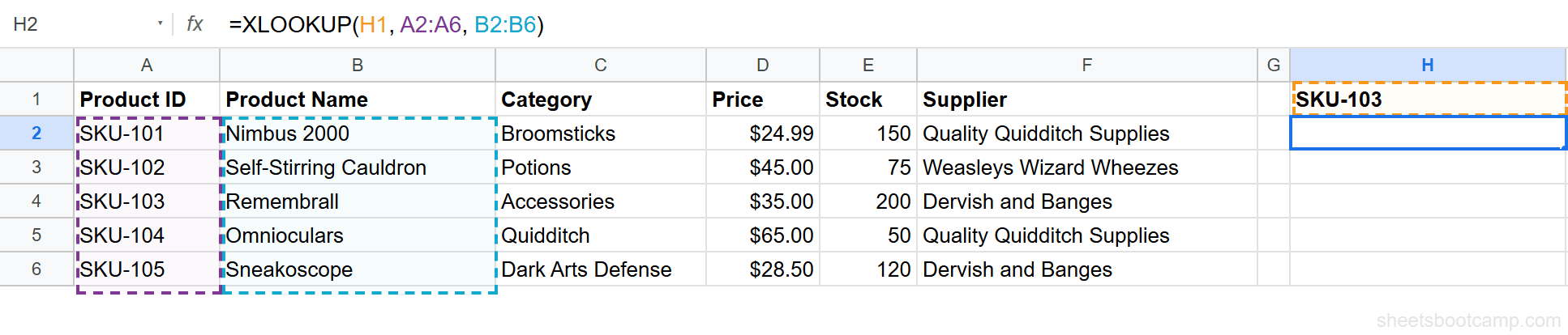
Select a cell for the result. Enter this formula:
=XLOOKUP(H1, A2:A6, B2:B6)H1is the search key — the Product ID to look upA2:A6is the lookup range — the column of Product IDs to search throughB2:B6is the result range — the column of Product Names to return from
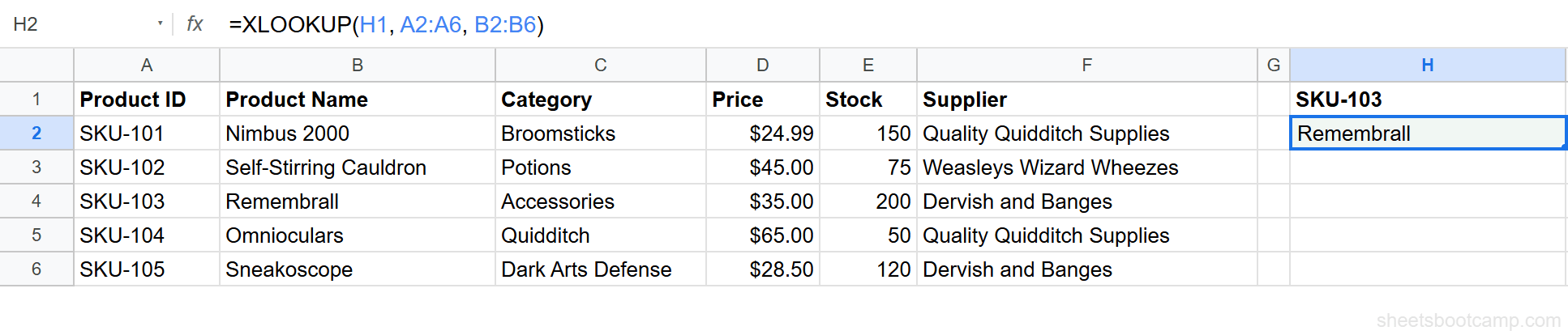
Press Enter. XLOOKUP finds SKU-103 in column A and returns “Remembrall” from column B.
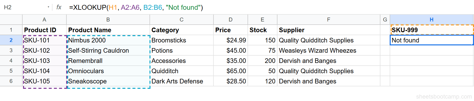
What if someone enters a Product ID that does not exist? By default, XLOOKUP returns a #N/A error. You can change this with the fourth parameter:
=XLOOKUP(H1, A2:A6, B2:B6, "Not found")Now if H1 contains an invalid SKU, the formula returns “Not found” instead of an error. No need to wrap the formula in IFERROR.
The built-in missing_value parameter is one of XLOOKUP’s biggest advantages over VLOOKUP. It keeps your formulas cleaner and easier to read.
XLOOKUP for Reverse Lookups
VLOOKUP can only return values to the right of the search column. XLOOKUP has no such limitation. The lookup_range and result_range are independent — you can search in any column and return from any other column.
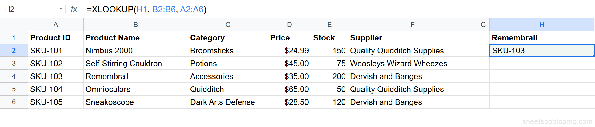
To look up a Product Name and return its Product ID (a left lookup), swap the ranges:
=XLOOKUP(H1, B2:B6, A2:A6)H1contains “Remembrall” (the product name)B2:B6is the lookup range (Product Names)A2:A6is the result range (Product IDs — to the left)
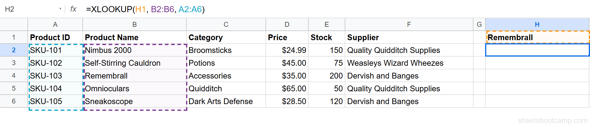
XLOOKUP returns SKU-103 from column A.
This is the single biggest reason to choose XLOOKUP over VLOOKUP. With VLOOKUP, a left lookup requires workarounds like INDEX MATCH. With XLOOKUP, you just change which ranges you point to.
XLOOKUP with Wildcards
Set match_mode to 2 to enable wildcard matching. Use * to match any sequence of characters and ? to match a single character.
This formula finds the first product name containing “Ext”:
=XLOOKUP("*Ext*", B2:B9, A2:A9, "Not found", 2)XLOOKUP matches “Extendable Ears” and returns its Product ID (SKU-106).
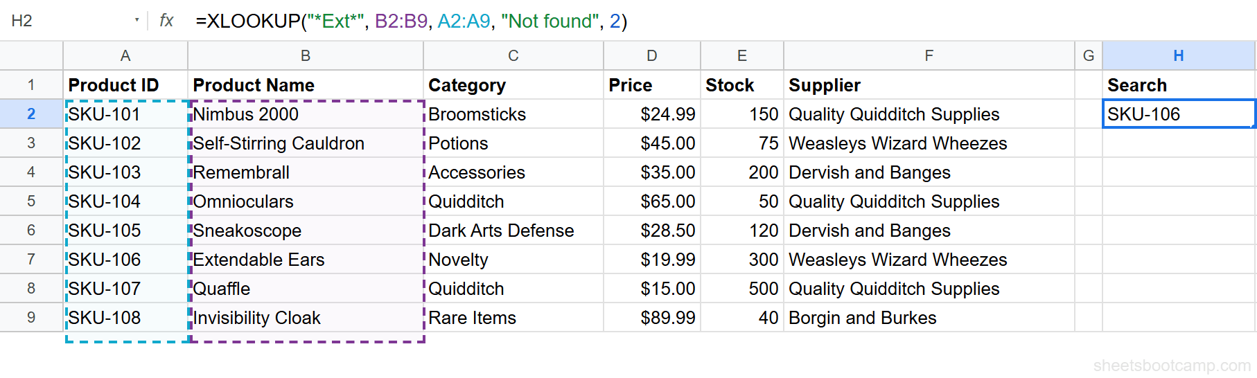
Wildcard matching is case-insensitive. "*ext*" and "*Ext*" return the same result.
XLOOKUP with Approximate Match
Set match_mode to -1 to find the exact match or next smaller value. This is ideal for bracket-based lookups like commission rates, tax brackets, or grade boundaries.
Here is a commission rate table. The goal is to find the correct rate for a $750 order:
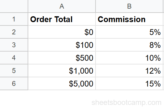
=XLOOKUP(D2, A2:A6, B2:B6, , -1)$750 falls between $500 and $1,000. With match_mode -1, XLOOKUP returns the rate for $500 (the next smaller value): 10%.
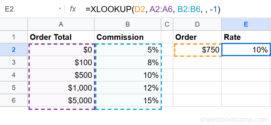
For approximate matching with match_mode -1, your lookup range must be sorted in ascending order (smallest to largest). Unsorted data produces incorrect results without any error.
Return Multiple Columns with XLOOKUP
XLOOKUP can return values from multiple columns in a single formula. Set the result_range to span more than one column, and the results spill across adjacent cells.
This formula looks up SKU-103 and returns both the Category (column C) and Price (column D):
=XLOOKUP(H1, A2:A6, C2:D6)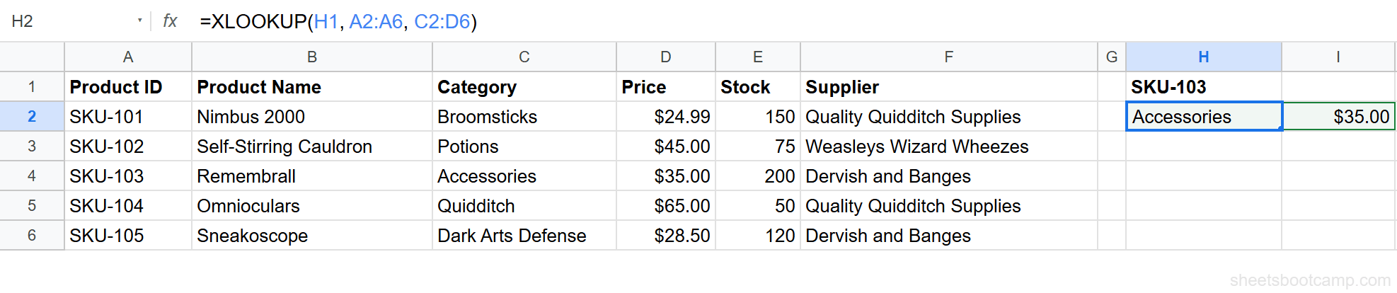
XLOOKUP returns “Accessories” in one cell and “$35.00” in the cell to its right. One formula, two results.
The cells to the right of your formula must be empty. If they contain data, XLOOKUP returns a #REF! error because it cannot spill the results.
XLOOKUP vs VLOOKUP
Here is how XLOOKUP compares to VLOOKUP on every major feature:
| Feature | VLOOKUP | XLOOKUP |
|---|---|---|
| Search direction | Right only | Any direction |
| Default match | Approximate (needs FALSE for exact) | Exact match |
| Error handling | Wrap in IFERROR | Built-in missing_value parameter |
| Column reference | Column index number (breaks if columns move) | Separate result range (stable) |
| Left lookup | Not possible without workarounds | Built-in |
| Wildcard mode | Supported | Dedicated match_mode 2 |
| Multiple column return | One column at a time | Multiple columns in one formula |
| Search direction | Top to bottom only | Top-to-bottom or bottom-to-top |
| Binary search | Not supported | Supported (search_mode 2 or -2) |
When to use XLOOKUP: New formulas. Any time you would reach for VLOOKUP, XLOOKUP does the same thing with fewer gotchas.
When to keep VLOOKUP: Existing formulas that already work. There is no need to rewrite a working VLOOKUP. Both functions will continue to work indefinitely.
XLOOKUP was added to Google Sheets in August 2022. If you share spreadsheets with people using older Google Sheets versions or Excel 2019 and earlier, they may not be able to use XLOOKUP formulas.
XLOOKUP vs INDEX MATCH
INDEX MATCH has been the go-to VLOOKUP alternative for years. How does XLOOKUP compare?
| Feature | INDEX MATCH | XLOOKUP |
|---|---|---|
| Syntax | Two nested functions | One function |
| Left lookup | Yes | Yes |
| Error handling | Wrap in IFERROR | Built-in |
| Multiple criteria | Possible with arrays | Possible with arrays |
| Availability | All versions of Google Sheets | August 2022 onward |
INDEX MATCH is still a strong choice. It works in every version of Google Sheets and Excel, and handles multiple criteria lookups well. XLOOKUP is simpler to write and read, especially for straightforward lookups.
If you already know INDEX MATCH, you do not need to switch. If you are learning lookup functions for the first time, start with XLOOKUP — the syntax is more intuitive.
Common XLOOKUP Errors
#N/A Error
XLOOKUP returns #N/A when the search key is not found. Common causes:
- Typos in the search key
- Extra spaces (use TRIM to clean data)
- Numbers stored as text (use VALUE to convert)
- The search key genuinely does not exist in the lookup range
Use the missing_value parameter to handle this gracefully: =XLOOKUP(A2, B:B, C:C, "Not found")
Mismatched Range Sizes
The lookup_range and result_range must have the same number of rows (for vertical lookups) or columns (for horizontal lookups). If they do not match, XLOOKUP returns an error.
Wrong Results with Approximate Match
If you use match_mode -1 or 1 on unsorted data, XLOOKUP returns incorrect results without showing an error. Always sort your lookup range when using approximate matching.
For more on fixing lookup errors, see the troubleshooting guide.
Tips for Using XLOOKUP
- Start simple. The first three parameters handle most lookups. Add match_mode and search_mode only when you need them.
- Use missing_value. Always set the fourth parameter to a friendly message like
"Not found"or0. This prevents#N/Aerrors from breaking downstream formulas like SUM or AVERAGE. - Lock ranges with $. Use absolute references (
$A$2:$A$100) when copying XLOOKUP formulas across multiple rows. This prevents the ranges from shifting. - Use binary search for large datasets. If your lookup range has thousands of rows and is already sorted, set search_mode to
2for faster performance.
Related Google Sheets Tutorials
- VLOOKUP: The Complete Guide — Covers the original lookup function in depth
- INDEX MATCH: The Complete Guide — The flexible two-function lookup alternative
- Fix VLOOKUP Errors — Troubleshoot #N/A, #REF!, and #VALUE! errors
- INDEX MATCH vs VLOOKUP — Detailed comparison of both approaches
- VLOOKUP for Beginners — Step-by-step starter guide for lookup functions