ARRAYFORMULA in Google Sheets: Complete Guide
Learn how to use ARRAYFORMULA in Google Sheets to apply a formula to an entire column from one cell. Step-by-step examples with IF, VLOOKUP, and more.
Sheets Bootcamp
March 29, 2026
ARRAYFORMULA in Google Sheets applies a formula to an entire column from a single cell. Instead of typing a formula in one row and dragging it down, you write it once and every row gets the result automatically.
This guide covers the ARRAYFORMULA syntax, a step-by-step tutorial with sales data, practical examples with IF and text functions, common errors, and tips for clean array formulas.
What Is ARRAYFORMULA?
ARRAYFORMULA takes a formula that normally calculates one cell and extends it across a range. You enter it in the first row, and results fill down the column without any manual copying.
This matters for three reasons. First, you maintain one formula instead of hundreds — edit it once and every row updates. Second, new rows added to the data range get calculated automatically when you use open-ended ranges like A2:A. Third, collaborators cannot accidentally delete or modify individual row formulas because the formula only exists in one cell.
ARRAYFORMULA Syntax
Here is the full ARRAYFORMULA syntax in Google Sheets:
=ARRAYFORMULA(array_formula)| Parameter | Required | Description |
|---|---|---|
| array_formula | Yes | A formula that uses range references instead of single cell references |
The formula inside ARRAYFORMULA must use ranges (A2:A9 or A2:A) instead of single cells (A2). When ARRAYFORMULA evaluates the expression, it applies the operation to every cell in the range and returns an array of results.
Use range references, not single cell references. =ARRAYFORMULA(A2*B2) calculates one cell. =ARRAYFORMULA(A2:A*B2:B) calculates every row. This is the most common mistake.
How to Use ARRAYFORMULA: Step-by-Step
Here is a sales records table with 8 transactions. The goal is to calculate the price per unit for every row using a single formula.

Add a “Price Per Unit” header in cell H1. Select cell H2 and enter this formula:
=ARRAYFORMULA(F2:F9/E2:E9)F2:F9is the Revenue columnE2:E9is the Units column- The division applies to every row in the range
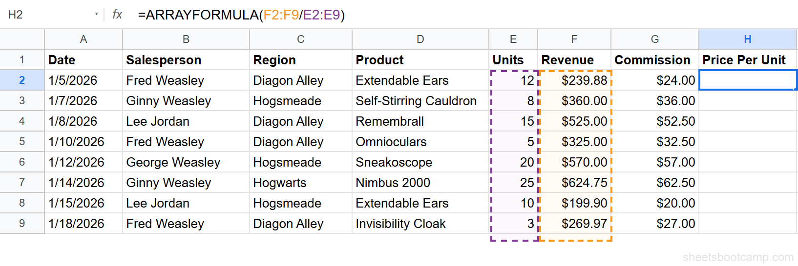
Press Enter. Column H fills with the price per unit for all 8 sales. The formula lives in H2 but produces results in H2 through H9.
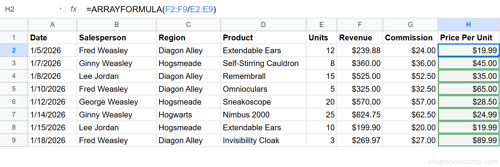
Row 2 shows $19.99 (Extendable Ears: $239.88 divided by 12 units). Row 7 shows $24.99 (Nimbus 2000: $624.75 divided by 25 units).
Cells H3 through H9 show results but contain no formula. If you click on H3, the formula bar is empty. The entire column is controlled by the single formula in H2.
The formula above uses a fixed range (F2:F9). To make it work with future rows, switch to an open-ended range — but blank rows will return divide-by-zero errors. Wrap the formula in IF to handle blanks:
=ARRAYFORMULA(IF(E2:E="", "", F2:F/E2:E))E2:Eis an open-ended range — it extends to every row in the sheetIF(E2:E="", "")returns an empty string for blank rowsF2:F/E2:Ecalculates the price per unit for rows with data
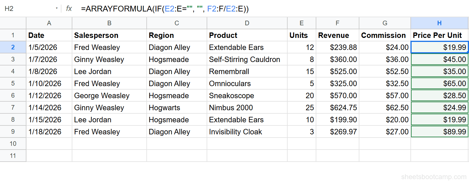
The IF wrapper is the standard pattern for production-ready array formulas. Without it, every blank row below your data shows an error.
Press Ctrl+Shift+Enter (Cmd+Shift+Enter on Mac) after typing any formula to wrap it in ARRAYFORMULA automatically. You do not need to type “ARRAYFORMULA(” manually.
ARRAYFORMULA Examples
Example 1: ARRAYFORMULA with IF for Categories
Classify each sale as “Gold,” “Silver,” or “Bronze” based on commission amount. Add a “Tier” header in column I.
=ARRAYFORMULA(IF(E2:E="", "", IF(G2:G>50, "Gold", IF(G2:G>30, "Silver", "Bronze"))))- Commission above $50: Gold (rows 4, 6, 7)
- Commission between $30.01 and $50: Silver (rows 3, 5)
- Commission $30 or below: Bronze (rows 2, 8, 9)
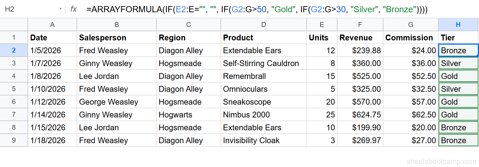
The outer IF(E2:E="", "") prevents the nested IF from evaluating blank rows. Every IF reference inside ARRAYFORMULA must use ranges, not single cells.
Example 2: ARRAYFORMULA with Text Functions
Combine the salesperson name and region into a single label. Add a “Sales Rep (Region)” header in column I.
=ARRAYFORMULA(IF(B2:B="", "", B2:B&" ("&C2:C&")"))This concatenates column B, a space and opening parenthesis, column C, and a closing parenthesis. Row 2 returns “Fred Weasley (Diagon Alley).”
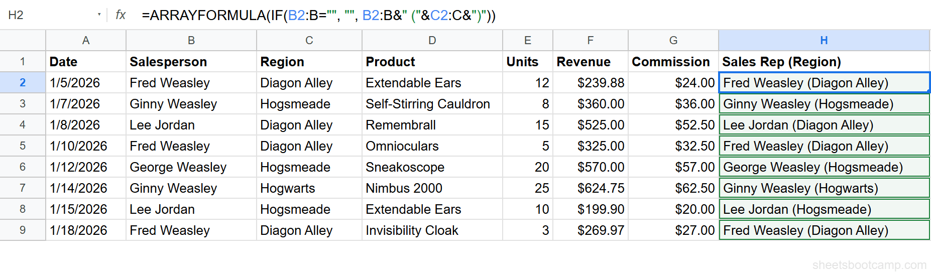
The & operator works inside ARRAYFORMULA the same way it works in a regular formula. You can also use CONCATENATE, UPPER, LOWER, LEFT, RIGHT, and other text functions inside ARRAYFORMULA.
Example 3: ARRAYFORMULA with VLOOKUP
ARRAYFORMULA extends VLOOKUP across an entire column. If you have product names in column D and need to look up their categories from a reference table, one formula handles every row:
=ARRAYFORMULA(IF(D2:D="", "", VLOOKUP(D2:D, Products!A:C, 3, FALSE)))Without ARRAYFORMULA, you would enter the VLOOKUP in one cell and drag it down. With ARRAYFORMULA, a single formula in the first row covers the entire column.
ARRAYFORMULA vs Dragging Formulas
| ARRAYFORMULA | Dragging Formulas | |
|---|---|---|
| Number of formulas | One formula in the first row | One formula per row |
| New rows | Covered automatically (with open-ended ranges) | Must drag formula to new rows manually |
| Editing | Edit once, all rows update | Must edit every row (or drag again) |
| Accidental deletion | Cannot delete individual row results | Any row formula can be deleted |
| Performance | Single calculation pass | Calculated row by row |
| Works with | Most functions (math, text, logical, lookup) | All functions |
Use ARRAYFORMULA when you have a calculated column that applies the same logic to every row. Use individual formulas when different rows need different formulas or when the function does not support array evaluation.
Common Errors and How to Fix Them
Only One Result Returned
The formula uses single cell references instead of ranges. =ARRAYFORMULA(F2/E2) returns one value. Change it to =ARRAYFORMULA(F2:F/E2:E) with range references.
This is the most common ARRAYFORMULA mistake. Every reference inside the formula must be a range for the array to expand.
#REF! — Output Range Blocked
ARRAYFORMULA fills results into the cells below it. If those cells already contain data or another formula, Google Sheets returns #REF!.
Fix: clear the cells below the ARRAYFORMULA, or move the formula to an empty column.
Blank Rows Showing Errors or Zeros
When using open-ended ranges like E2:E, blank rows get calculated too. Dividing empty cells produces errors. Comparing empty cells produces unwanted results.
Fix: wrap the formula in IF to skip blank rows:
=ARRAYFORMULA(IF(E2:E="", "", your_formula_here))Check the column that best indicates whether a row has data. Usually this is the first data column (like Date or ID).
Always use the IF-blank-check pattern for open-ended array formulas. It prevents errors in blank rows and keeps your sheet clean.
Circular Dependency
ARRAYFORMULA cannot reference its own output column. If the formula is in column H and it references H2:H, Google Sheets detects a circular reference.
Fix: make sure the formula only references input columns, not the column where the results appear.
Tips and Best Practices
- Always wrap in IF for blank rows. The pattern
=ARRAYFORMULA(IF(A2:A="", "", your_formula))is the standard. Use it every time you use an open-ended range. - Place the formula in the first data row. ARRAYFORMULA goes in row 2 (the first row after headers). It fills down from there. Placing it in a middle row leaves gaps above.
- Use open-ended ranges for growing data.
A2:Ainstead ofA2:A100. Open-ended ranges automatically include new rows added to the sheet. - Not all functions work inside ARRAYFORMULA. Most math, text, and logical functions work. Some functions like IMPORTRANGE and GOOGLEFINANCE do not expand inside ARRAYFORMULA. Test your formula first.
- One ARRAYFORMULA per column. If H2 contains an ARRAYFORMULA that fills down to H100, do not put another formula in H50. The first formula controls the entire column.
Related Google Sheets Tutorials
- IF Function: Complete Guide — Conditional logic that pairs with ARRAYFORMULA for entire-column IF statements
- VLOOKUP: Complete Guide — Look up values from another table, expandable to whole columns with ARRAYFORMULA
- FILTER Function: Complete Guide — Return rows matching conditions as a dynamic array
- QUERY Function: Complete Guide — SQL-like queries for filtering, sorting, and aggregating data
Frequently Asked Questions
What does ARRAYFORMULA do in Google Sheets?
ARRAYFORMULA takes a formula that normally works on a single cell and applies it to an entire range of cells. You enter the formula once in the first cell, and it fills results down the column automatically.
How do I apply a formula to an entire column in Google Sheets?
Wrap your formula in ARRAYFORMULA and use column ranges instead of single cell references. For example, =ARRAYFORMULA(A2:A*B2:B) multiplies every row in columns A and B. Use an open-ended range like A2:A to include future rows.
Why does my ARRAYFORMULA only return one result?
Your formula uses single cell references instead of ranges. =ARRAYFORMULA(A2*B2) only calculates one cell. Change it to =ARRAYFORMULA(A2:A*B2:B) with range references to get results for every row.
Can I use ARRAYFORMULA with IF?
Yes. =ARRAYFORMULA(IF(A2:A>100, "High", "Low")) applies the IF logic to every row in column A. Wrap ARRAYFORMULA around the entire IF statement and use ranges for all cell references inside the IF.
Does ARRAYFORMULA slow down Google Sheets?
ARRAYFORMULA is more efficient than individual formulas in each row because Google Sheets processes the entire range in one calculation pass. Large sheets with thousands of rows may see minor slowdowns, but ARRAYFORMULA is faster than the equivalent row-by-row formulas.
What is the keyboard shortcut for ARRAYFORMULA?
Press Ctrl+Shift+Enter (Cmd+Shift+Enter on Mac) after typing a formula. Google Sheets wraps it in ARRAYFORMULA automatically. You can also type ARRAYFORMULA( ) manually.