
=FILTER(A2:F9, C2:C9="Surveillance") returns every row where column C equals Surveillance. The first argument is the data to return, and every argument after it is a condition the same height as that data. Commas between conditions mean AND, a + between them means OR, and the result spills down on its own and updates the moment the source data changes.
beginner 7 min read
FILTER Function in Google Sheets: Complete Guide
Learn how to use the FILTER function in Google Sheets to extract rows matching conditions. Covers multiple criteria, AND/OR logic, and real examples.
SB
Sheets Bootcamp
March 12, 2026 · Updated August 17, 2026
Table of Contents
Quick Answer
The FILTER function in Google Sheets returns rows from a range that match one or more conditions. It creates a dynamic filtered view without modifying your source data, the results update automatically whenever the original data changes.
This guide covers the FILTER syntax, step-by-step examples with single and multiple conditions, AND vs OR logic, combining FILTER with SORT, common errors, and a comparison with QUERY.
FILTER Syntax
Here is the full FILTER syntax in Google Sheets:
Formula
=FILTER(range, condition1, [condition2, ...]) | Parameter | Required | Description |
|---|---|---|
| range | Yes | The range of data to filter and return |
| condition1 | Yes | A column or row of TRUE/FALSE values (same height as range) |
| condition2, … | No | Additional conditions. Each extra condition acts as AND logic |
Important
Each condition must produce a column of TRUE or FALSE values the same size as the range. Write conditions as comparisons against a column: C2:C9="Surveillance" produces TRUE for each row where column C equals “Surveillance” and FALSE for the rest.
FILTER returns every row where all conditions evaluate to TRUE. The results spill into adjacent cells below the formula.
How to Use FILTER: Step-by-Step
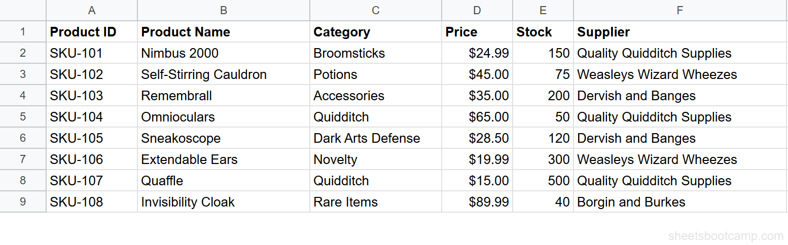
Here is a product inventory table with 8 products. The goal is to filter products in the “Surveillance” category.
| A | B | C | D | E | F | |
|---|---|---|---|---|---|---|
| 1 | Product ID | Product Name | Category | Price | Stock | Supplier |
| 2 | SKU-101 | Magnifying Glass | Optics | $24.99 | 150 | Baker Street Supply Co. |
| 3 | SKU-102 | Forensic Chemistry Set | Laboratory | $45.00 | 75 | Watson Medical Supplies |
| 4 | SKU-103 | Pocket Watch | Accessories | $35.00 | 200 | Strand Curiosities |
| 5 | SKU-104 | Field Binoculars | Surveillance | $65.00 | 50 | Baker Street Supply Co. |
| 6 | SKU-105 | Cipher Decoder | Cryptography | $28.50 | 120 | Strand Curiosities |
| 7 | SKU-106 | Deerstalker Cap | Apparel | $30.00 | 90 | Regent Timeworks |
| 8 | SKU-107 | Evidence Bag Kit | Surveillance | $15.00 | 500 | Baker Street Supply Co. |
| 9 | SKU-108 | Brass Telescope | Optics | $42.00 | 85 | Baker Street Supply Co. |
1
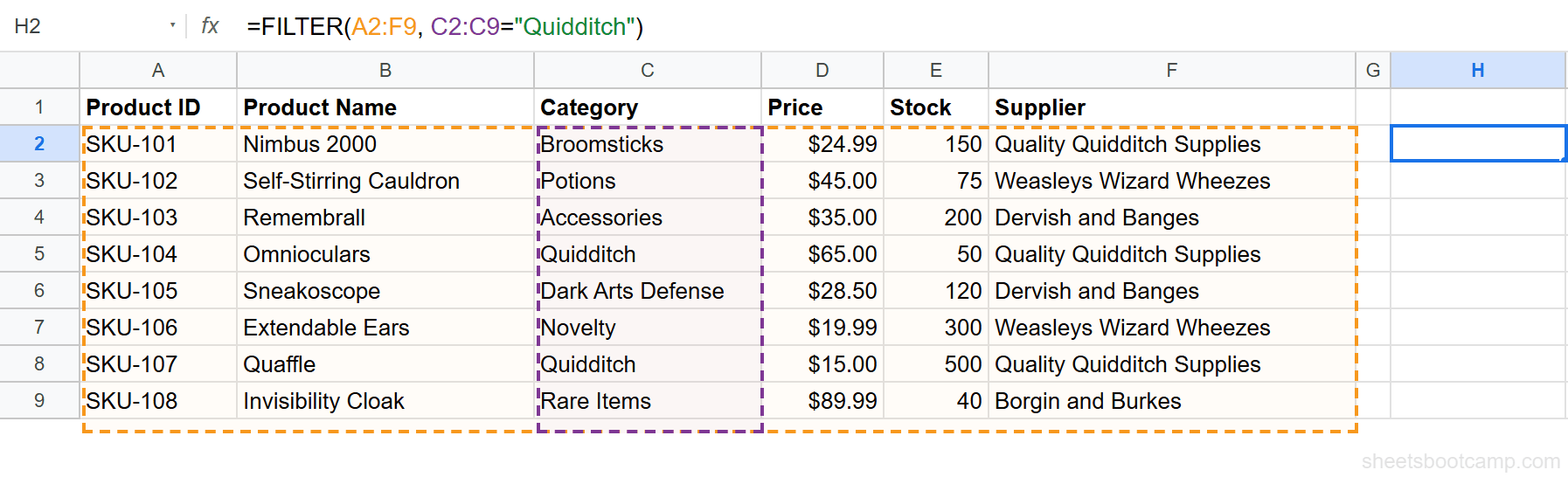
Select cell H2. Enter this formula:
Formula
=FILTER(A2:F9, C2:C9="Surveillance") A2:F9is the range, all data rows across all columnsC2:C9="Surveillance"is the condition, return rows where Category equals “Surveillance”
2
Press Enter. FILTER returns two rows: Field Binoculars (SKU-104) and Evidence Bag Kit (SKU-107). Both have “Surveillance” in the Category column.

The results spill into cells H2:M3 automatically. FILTER always returns the full rows (or whichever columns you included in the range argument).
3
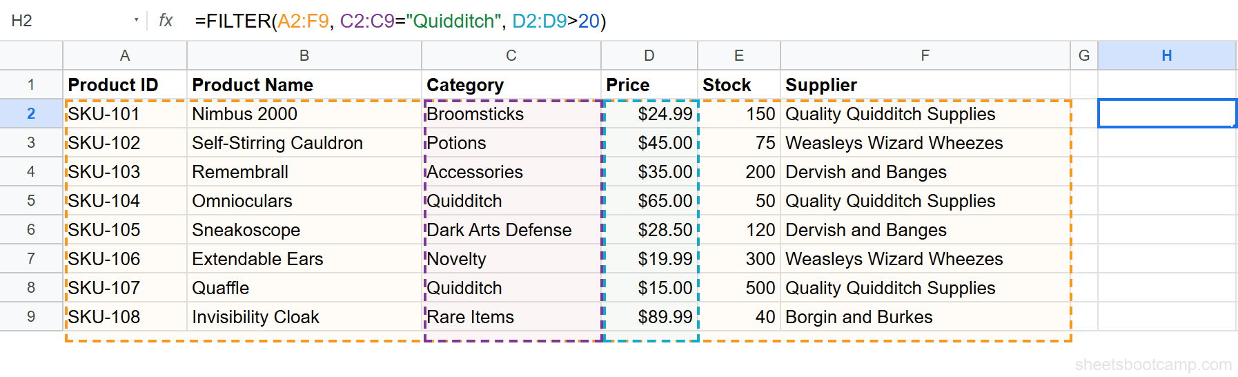
To filter Surveillance products priced above $20, add a second condition:
Formula
=FILTER(A2:F9, C2:C9="Surveillance", D2:D9>20) Each condition separated by a comma acts as AND logic, both must be TRUE for a row to appear.
4
Only Field Binoculars ($65.00) matches both conditions. The Evidence Bag Kit ($15.00) is excluded because its price is not above $20.

Tip
You can add as many comma-separated conditions as you need. Each one narrows the results further. Think of commas as AND.
FILTER with OR Conditions
Comma-separated conditions are AND logic. For OR logic, use the + operator and wrap the combined condition in parentheses.
This formula filters products in the “Surveillance” OR “Optics” category:
Formula
=FILTER(A2:F9, (C2:C9="Surveillance")+(C2:C9="Optics")) The + operator combines the two conditions with OR logic. A row appears if either condition is TRUE.

FILTER returns four rows: Magnifying Glass and Brass Telescope (Optics), plus Field Binoculars and Evidence Bag Kit (Surveillance).
Important
The parentheses around each condition are required when using + for OR. Without them the formula does not misbehave quietly, it fails: =FILTER(A2:F9, C2:C9="Surveillance"+C2:C9="Optics") returns #N/A. Sheets reads "Surveillance"+C2:C9 first, and adding text to a range is not a comparison at all, so nothing is left for FILTER to test.
You can combine AND and OR in the same formula. Use + for OR within parentheses, and commas for AND between conditions:
Formula
=FILTER(A2:F9, (C2:C9="Surveillance")+(C2:C9="Optics"), D2:D9>20) This returns Surveillance or Optics products priced above $20. The Evidence Bag Kit ($15.00) is excluded.
FILTER Examples
Example 1: Filter by Price Range
To find products priced between $20 and $50:
Formula
=FILTER(A2:F9, D2:D9>=20, D2:D9<=50) Both price conditions use commas (AND logic). The result includes every product where the price is at least $20 and at most $50.
Example 2: Filter with Partial Text Match
FILTER conditions are exact comparisons by default. To filter rows containing specific text, combine FILTER with SEARCH and ISNUMBER:
Formula
=FILTER(A2:F9, ISNUMBER(SEARCH("Baker", F2:F9))) SEARCH("Baker", F2:F9) returns a number (the position) when “Baker” appears in the Supplier column, and an error when it does not. ISNUMBER converts those results to TRUE/FALSE. The formula returns the four products supplied by Baker Street Supply Co.: Magnifying Glass, Field Binoculars, Evidence Bag Kit and Brass Telescope.
Tip
Point the search at the column that actually contains the word. SEARCH looks inside one range only, so searching the Supplier column for a category name like “Surveillance” matches nothing and the whole formula returns #N/A. To match a category by partial text, aim it at column C instead: =FILTER(A2:F9, ISNUMBER(SEARCH("Surveillance", C2:C9))).
Example 3: FILTER + SORT
FILTER results come back in the same order as the source data. To sort the filtered results, wrap FILTER inside SORT:
Formula
=SORT(FILTER(A2:F9, C2:C9="Surveillance"), 4, TRUE) This filters Surveillance products and sorts them by column 4 (Price) in ascending order.

Tip
The column number in SORT refers to the position within the filtered output, not the original sheet. Column 4 in the FILTER result is Price (the fourth column of A2:F9).
FILTER vs QUERY
Both FILTER and QUERY return subsets of your data, but they work differently.
| Feature | FILTER | QUERY |
|---|---|---|
| Syntax | Cell references + comparison operators | Text-based query language (SQL-like) |
| Multiple conditions | Commas for AND, + for OR | WHERE with AND/OR keywords |
| Sorting | Wrap in SORT | Built-in ORDER BY |
| Grouping / aggregation | Not supported (use SUMIF, COUNTIF) | Built-in GROUP BY, SUM, COUNT, AVG |
| Column selection | Change the range argument | SELECT specific columns |
| Learning curve | Lower, standard formula syntax | Higher, requires query language syntax |
Use FILTER when you need to grab rows matching conditions. It is faster to write and easier to read for straightforward filtering.
Use QUERY when you need to group, aggregate, sort, or select specific columns in one formula. QUERY handles more complex data operations in a single step.
Common Errors and How to Fix Them
#N/A: No Matching Rows
FILTER returns #N/A when no rows match all conditions. This is not a formula error, it means the filter worked correctly but found nothing.
Wrap the formula in IFERROR to return a message instead:
Formula
=IFERROR(FILTER(A2:F9, C2:C9="Wands"), "No results found") 
#N/A: Condition Size Mismatch
Each condition must have the same number of rows as the range. If A2:F9 has 8 rows but your condition references C2:C5 (4 rows), FILTER returns #N/A. It reads the same either way round: a 4-row range against an 8-row condition returns #N/A too.
Fix: make sure every condition column covers the same row range as the data.
Warning
A mismatch in the row count is loud. A mismatch in which rows are covered is silent. =FILTER(A2:F9, C1:C8="Surveillance") has 8 data rows and an 8-row condition, so Sheets is satisfied and returns rows, but the condition is shifted up by one and the answer is Cipher Decoder and Brass Telescope, neither of which is a Surveillance product. Check that your condition starts on the same row as your data, not just that it is the same height.
#REF!: Spill Conflict
FILTER results spill into cells below the formula. If those cells already contain data, FILTER returns #REF!.
Fix: clear the cells below and to the right of the formula, or move the formula to an empty area.
Tip
Place FILTER formulas in a separate area of your sheet, away from the source data. This prevents spill conflicts and keeps your layout clean.
Tips and Best Practices
- Use cell references for conditions. Instead of hardcoding
"Surveillance"in the formula, reference a cell:=FILTER(A2:F9, C2:C9=H1). Change H1 to filter by any category without editing the formula. - Combine FILTER with SORT, UNIQUE, or INDEX. FILTER returns an array, so you can nest it inside other functions.
=UNIQUE(FILTER(B2:B9, C2:C9="Surveillance"))returns unique product names. - FILTER can return columns too. To filter columns instead of rows, orient the condition as a row:
=FILTER(A1:F1, A2:F2>50). Be careful what you compare against, though. That formula returns five of the six headers, not just Stock, because in Google Sheets any text value counts as greater than any number, so"SKU-101">50is TRUE. A numeric comparison across a row only behaves the way you expect when every cell in that row is a number. - FILTER results are dynamic. When source data changes, the filtered results update automatically. There is no need to re-run or refresh the formula.
Related Google Sheets Tutorials
- QUERY Function: Complete Guide: Text-based query language for filtering, sorting, and aggregating data
- VLOOKUP: Complete Guide: Look up a single value from a table by searching the first column
- XLOOKUP: Complete Guide: The modern lookup function with built-in error handling
- SUMIF and SUMIFS: Add values that match conditions without returning full rows
Frequently Asked Questions
What does the FILTER function do in Google Sheets?
The FILTER function returns rows or columns from a range that match one or more conditions. The results appear in adjacent cells automatically. Unlike the Data > Create a filter menu, FILTER is a formula that works anywhere in your spreadsheet.
How do I use FILTER with multiple conditions?
Add each condition as an additional argument separated by commas. Each comma-separated condition acts as AND logic. For OR logic, add conditions with + instead and wrap the combined condition in parentheses.
What is the difference between FILTER and QUERY?
FILTER uses cell references and comparison operators for conditions. QUERY uses a text-based query language similar to SQL. FILTER is faster to write for straightforward filtering. QUERY handles complex operations like GROUP BY, ORDER BY, and calculated columns.
Why does FILTER return #N/A?
FILTER returns #N/A for two different reasons. Either no rows matched your conditions, or a condition is not the same height as the range, for example an 8-row range against a 4-row condition. Both produce #N/A, not #VALUE!. Wrap the formula in IFERROR to return a custom message instead: =IFERROR(FILTER(A2:F9, C2:C9="Surveillance"), "No results found").
Can FILTER return specific columns instead of entire rows?
Yes. Change the first argument to include only the columns you want. For example, =FILTER(B2:B9, C2:C9="Surveillance") returns only the Product Name column for matching rows.
Does FILTER update automatically when data changes?
Yes. FILTER is a formula, so it recalculates every time the source data changes. If you add, edit, or delete rows in the source range, the filtered results update automatically.
You've googled this formula before. Probably more than once.
The Bootcamp is a real Google Sheet that grades every formula the moment you press Enter. 193 exercises across 9 modules, the 10% of Sheets that does 90% of the work. One payment of $29.
Get It for $29 Get the Bootcamp for $2930-day refund. Reply to any email and you get your money back.
Not ready to pay? Try Basic Training free →