Conditional Formatting in Google Sheets: Guide
Learn how to use conditional formatting in Google Sheets to highlight cells by value, color-code data, and create custom formula rules. Step-by-step examples.
Sheets Bootcamp
February 18, 2026
Conditional formatting in Google Sheets changes the appearance of cells based on rules you define. Instead of manually coloring cells, you set conditions — like “highlight values above 400” or “turn the row blue when the region is Hogwarts” — and Sheets applies the formatting automatically.
This guide walks through how to set up conditional formatting rules, use color scales, write custom formula rules, and manage multiple rules on the same range.
In This Guide
- What Is Conditional Formatting?
- How to Apply Conditional Formatting: Step-by-Step
- Conditional Formatting Rule Types
- Custom Formula Rules
- Practical Examples
- Managing Multiple Rules
- Common Mistakes and Fixes
- Tips and Best Practices
- Related Google Sheets Tutorials
- FAQ
What Is Conditional Formatting?
Conditional formatting automatically changes how a cell looks — its background color, text color, bold, italic, or strikethrough — based on a rule. The cell’s value doesn’t change, only its appearance.
This is useful for:
- Spotting high or low values at a glance (revenue above a threshold)
- Color-coding categories (regions, status labels, priority levels)
- Flagging problems (overdue dates, missing data, duplicate entries)
You define the rule once, and Sheets applies it across the entire range. When the data changes, the formatting updates automatically.
Without conditional formatting, you’d have to scan every cell in a column to find the values that matter — or manually paint each cell green, yellow, or red. That works for 10 rows. It falls apart at 500. Conditional formatting scales because the rules stay active no matter how many rows get added later.
How to Apply Conditional Formatting: Step-by-Step
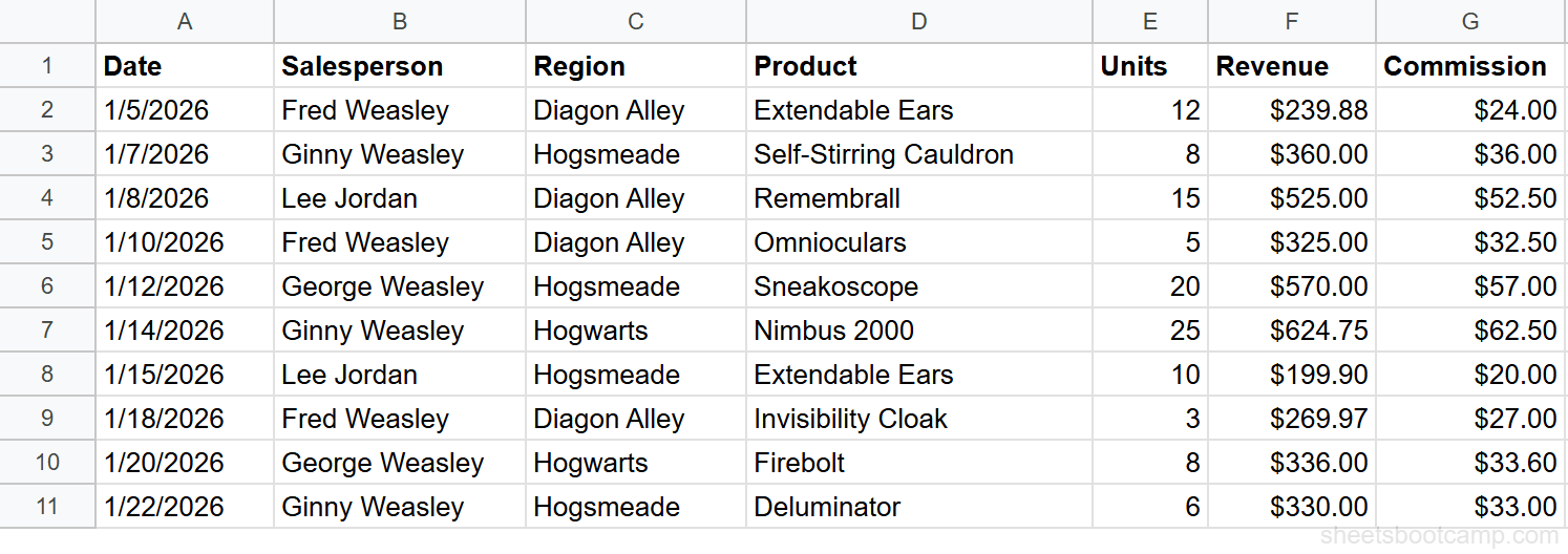
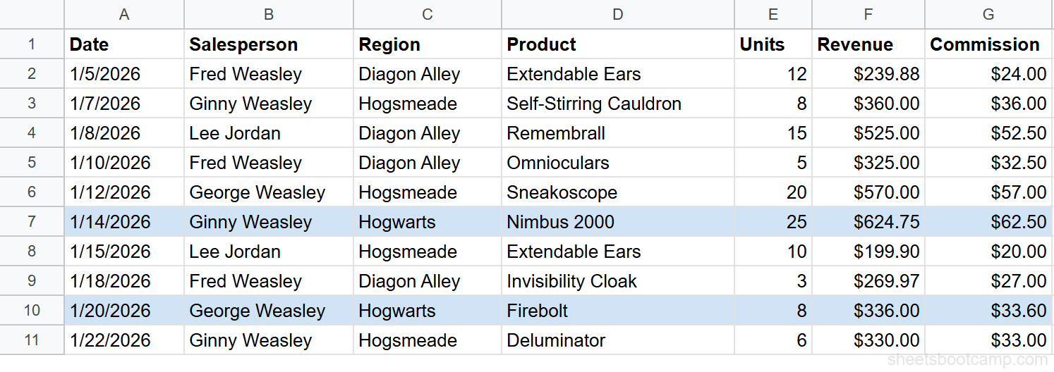
We’ll use a sales records table with 10 transactions. The goal: highlight revenue values above $400 in green.
Sample Data
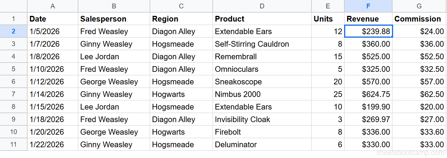
Select the range to format
Highlight cells F2 through F11 — the Revenue column, excluding the header. The range you select determines which cells the rule evaluates.
Open conditional formatting
Go to Format > Conditional formatting in the menu bar. The conditional format rules panel opens on the right side of the screen.
The “Apply to range” field should show F2:F11. If it doesn’t, you can type the range manually.
Set the rule condition
Under Format rules, click the dropdown that says “Is not empty” (the default). Select Greater than from the list, then enter 400 in the value field.
Choose the formatting style
Below the rule condition, you’ll see formatting options. Click the paint bucket icon and choose a green fill color. You can also change the text color, add bold, or apply italic — but for this example, a green background is enough.
Click Done to apply the rule.
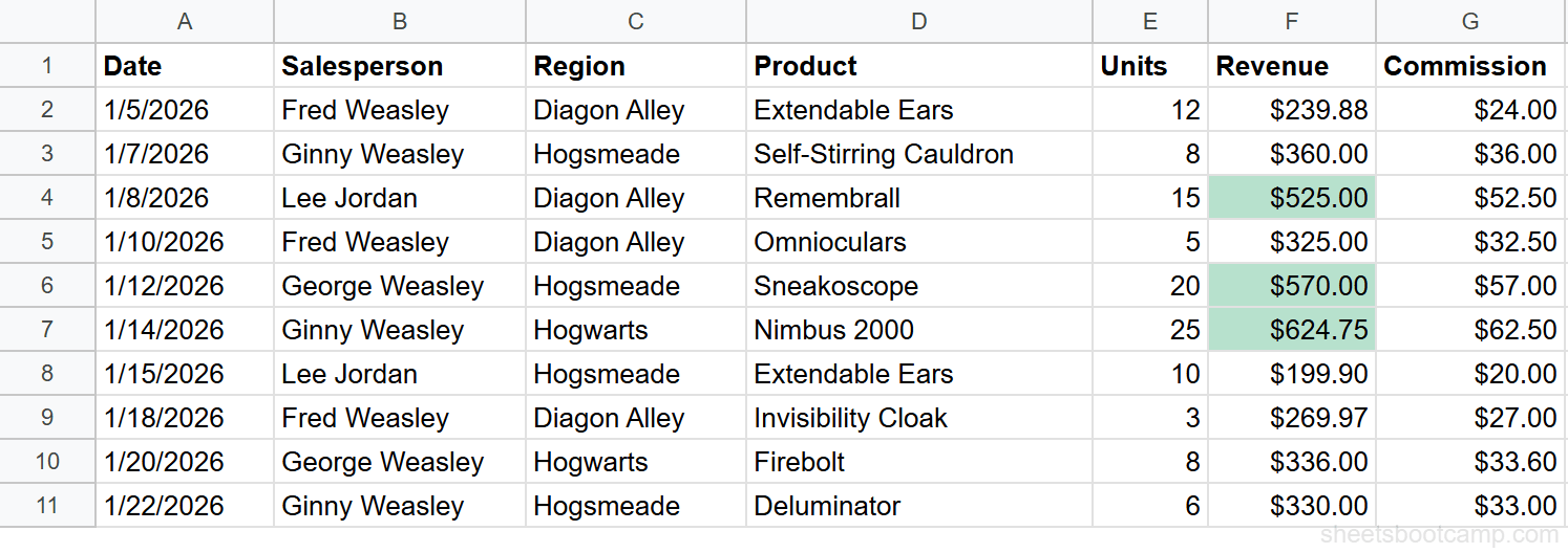
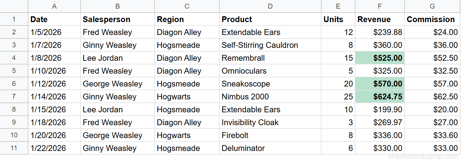
Review the result
Three cells are now highlighted green: Lee Jordan’s $525.00 (row 4), George Weasley’s $570.00 (row 6), and Ginny Weasley’s $624.75 (row 7). Every other cell in the Revenue column stays white.
To edit a rule later, go to Format > Conditional formatting and click on the rule in the panel. To add a second rule to the same range, click “Add another rule.”
Conditional Formatting Rule Types
Google Sheets provides two categories of built-in rules: single color and color scale.
Single Color Rules
Single color rules apply one formatting style (background color, text color, bold, etc.) when a condition is met. These are the most common rules.
| Rule Type | What It Does | Example |
|---|---|---|
| Is empty / Is not empty | Checks if a cell has content | Highlight blank cells to flag missing data |
| Text contains / Text does not contain | Matches partial text | Highlight cells containing “Hogwarts” |
| Text starts with / Text ends with | Matches the beginning or end of text | Highlight product names starting with “N” |
| Text is exactly | Matches the complete cell value | Highlight cells that say exactly “Diagon Alley” |
| Greater than / Less than | Compares against a numeric threshold | Highlight revenue above $400 |
| Greater than or equal to / Less than or equal to | Inclusive comparison | Highlight units of 10 or more |
| Is between / Is not between | Checks if a value falls in a range | Highlight revenue between $300 and $500 |
| Date is | Checks for specific date conditions | Highlight dates in the past week |
| Custom formula is | Uses any formula that returns TRUE/FALSE | The most flexible option (covered below) |
Color Scale
Color scale rules create a gradient across the selected range. Instead of one color for “pass” and nothing for “fail,” every cell gets a shade based on where its value falls between the minimum and maximum.
You pick two or three colors (min, midpoint, max), and Sheets interpolates the gradient automatically. This works well for numeric data where you want to see relative differences at a glance.
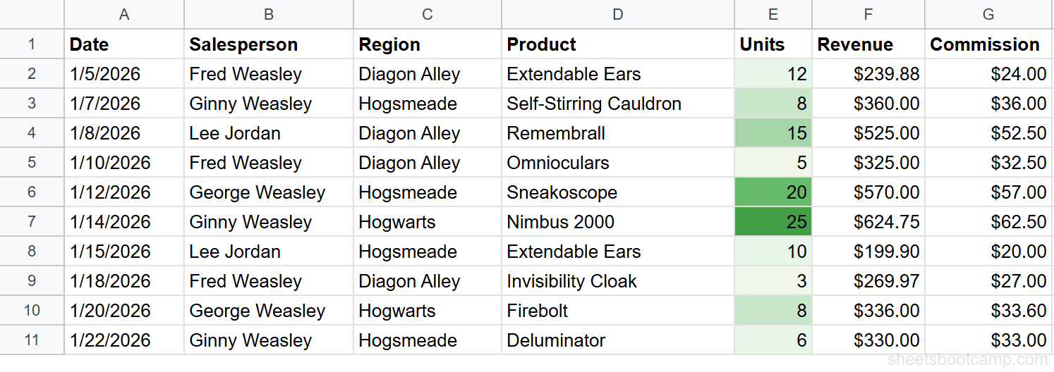
In this example, the Units column (E2:E11) uses a green color scale. Ginny Weasley’s 25 units is the darkest green, while Fred Weasley’s 3 units (Invisibility Cloak) is the lightest. Every other cell falls somewhere in between.
To set up a color scale:
- Select the numeric range (e.g., E2:E11)
- Open Format > Conditional formatting
- Under “Format rules,” switch to the Color scale tab
- Choose a preset gradient or set custom min/max colors
- Click Done
Google Sheets offers two-color and three-color scales. A three-color scale adds a midpoint — for example, red at the minimum, yellow at the midpoint, and green at the maximum. This is useful for data where you want to distinguish between “bad,” “neutral,” and “good” instead of a simple low-to-high gradient.
Color scale only works with numeric data. If the range contains text, those cells get no color. Mixed data types in a color scale range can produce unexpected gaps.
Custom Formula Rules
Custom formula rules are the most powerful option. Instead of picking from a preset dropdown, you write a formula that returns TRUE or FALSE. When the formula returns TRUE for a cell, that cell gets the formatting.
The Pattern
Select your range, choose Custom formula is from the rule type dropdown, and enter a formula. The formula is evaluated relative to the first cell in the “Apply to range” — so if your range starts at A2, write the formula as if you’re in cell A2.
Example 1: Highlight Entire Rows by Region
Apply this rule to the range A2:G11 to highlight every column in rows where the region is “Hogwarts”:
=$C2="Hogwarts"The $C locks the column reference to C (Region), but the row reference 2 is relative — it shifts to 3, 4, 5, and so on for each row. This means the formula checks column C for every row and applies the formatting across all columns in that row.
Rows 7 (Ginny Weasley, Nimbus 2000) and 10 (George Weasley, Firebolt) are highlighted because their Region column contains “Hogwarts.”
For a detailed walkthrough of this technique, see conditional formatting based on another cell and highlighting entire rows.
Example 2: Highlight Cells Above the Average
Apply this rule to F2:F11 to highlight revenue values that exceed the column average:
=F2>AVERAGE($F$2:$F$11)The $F$2:$F$11 uses absolute references so the average range doesn’t shift as the formula evaluates each cell. The F2 at the start is relative — it adjusts for each row.
The average revenue across all 10 rows is $378.05. Three cells exceed that: $525.00, $570.00, and $624.75.
Key Concept: Relative vs. Absolute References
The most common mistake with custom formulas is getting the $ signs wrong.
$C2— Column locked, row shifts. Use this when checking one column across multiple rows (like the region example).C$2— Row locked, column shifts. Use this when comparing against a specific row.$C$2— Both locked. Use this for fixed references (like the AVERAGE range).C2— Both shift. Use this when the formula should adapt to both the row and column of each cell.
Test your custom formula in a regular cell first. Enter the formula in a cell, verify it returns TRUE or FALSE for the expected rows, then copy it into the conditional formatting rule. This saves time debugging invisible formula errors.
For more custom formula patterns, see the full guide on conditional formatting with custom formulas.
Practical Examples
Example 1: Color-Code Revenue Tiers
Three rules applied to F2:F11, in this order:
- Greater than 500 → Green background (
#b7e1cd) - Is between 300 and 500 → Yellow background (
#fce8b2) - Less than 300 → Red background (
#f4c7c3)
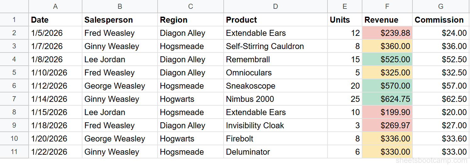
The result is a traffic-light pattern: green for high revenue ($525, $570, $624.75), yellow for mid-range ($360, $325, $336, $330), and red for low values ($239.88, $199.90, $269.97).
When stacking multiple rules on the same range, add them in order from most specific to least specific. Sheets evaluates rules top to bottom — the first matching rule determines the formatting.
Example 2: Highlight the Top 3 Values
Use a custom formula on F2:F11:
=F2>=LARGE($F$2:$F$11, 3)The LARGE function returns the 3rd-largest value in the range ($525.00). Any cell with revenue greater than or equal to that value gets highlighted. This catches $525.00, $570.00, and $624.75.
Example 3: Above-Average Rows (Custom Formula)
Use a custom formula on the entire data range A2:G11:
=$F2>AVERAGE($F$2:$F$11)This highlights the entire row — not just the Revenue cell — for any transaction where revenue exceeds the $378.05 average. The $F2 locks to the Revenue column while the row shifts for each row evaluated.
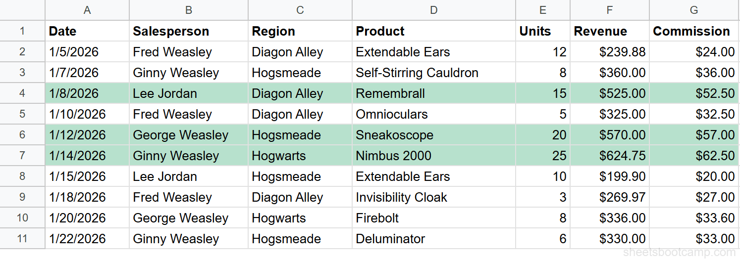
Three rows are highlighted: Lee Jordan ($525.00), George Weasley ($570.00), and Ginny Weasley ($624.75).
Example 4: Highlight Duplicate Salesperson Names
Use a custom formula on B2:B11 to flag any salesperson name that appears more than once:
=COUNTIF($B$2:$B$11, B2)>1COUNTIF counts how many times the value in B2 appears across the full range. If the count exceeds 1, the cell has a duplicate. In our sales data, every salesperson appears multiple times, so all cells would be highlighted. This pattern is more useful on columns where duplicates are unexpected — like order IDs or email addresses.
For a detailed walkthrough of duplicate detection, including highlighting the first occurrence vs. all occurrences, see highlighting duplicates in Google Sheets.
Example 5: Flag Dates Older Than a Threshold
Use a custom formula on A2:A11 to highlight dates before January 15, 2026:
=A2<DATE(2026, 1, 15)Cells with dates 1/5/2026, 1/7/2026, 1/8/2026, and 1/10/2026 are highlighted because they fall before January 15. The DATE function creates a proper date value for the comparison — don’t compare against a text string like “1/15/2026,” which can break when regional date formats differ.
This pattern adapts to dynamic thresholds too. Replace the DATE function with =A2<TODAY()-30 to highlight dates more than 30 days in the past. For more date-based patterns, see conditional formatting with dates.
Managing Multiple Rules
When you apply more than one rule to the same range, order matters.
Rule Priority
Google Sheets evaluates rules from top to bottom in the conditional format rules panel. The first rule that matches a cell determines its formatting.
If two rules both match a cell, the first rule’s formatting applies. To reorder rules, drag them up or down in the panel.
For example, take the three revenue-tier rules from earlier. If “Greater than 300” (yellow) is listed above “Greater than 500” (green), a cell with $570 matches both rules — but it turns yellow because that rule is first. The fix: drag “Greater than 500” above “Greater than 300” so the more specific rule gets checked first. As a general principle, put the most specific conditions at the top and the broadest conditions at the bottom.
Editing and Deleting Rules
- Edit: Open Format > Conditional formatting, click the rule you want to change, modify the condition or style, and click Done.
- Delete one rule: Click the trash icon next to the rule in the panel.
- Delete all rules: Scroll to the bottom of the panel and click “Remove all rules.”
Deleting a rule removes the formatting immediately. If cells looked green because of a rule and you delete it, they go back to their default appearance. Conditional formatting never modifies the actual cell values — only the display.
Performance
Each conditional formatting rule is evaluated for every cell in the range. Ten rules on a range of 10,000 cells means 100,000 evaluations. On large spreadsheets, this can cause noticeable lag.
Keep rules targeted to specific ranges instead of applying them to entire columns (A:A). Delete rules you no longer need. If the spreadsheet feels slow, check Format > Conditional formatting and look for leftover rules on large ranges.
Common Mistakes and Fixes
Wrong “Apply to Range”
You set up a rule but only one cell changes color. This usually means you selected a single cell instead of the full range before opening conditional formatting.
Fix: Open the rule, click the “Apply to range” field, and change it to the range you intended (e.g., F2:F11 instead of F2).
Relative vs. Absolute Reference in Custom Formulas
Your custom formula highlights the wrong rows, or highlights all rows instead of specific ones.
Fix: Check your $ signs. For a row-by-row check against a specific column, lock the column: =$C2="Hogwarts". For a fixed reference like an average, lock both: AVERAGE($F$2:$F$11).
Rule Order Conflicts
Two rules match the same cell, and the wrong color appears. For example, a “Greater than 300” rule (yellow) is above a “Greater than 500” rule (green), so $525 shows yellow instead of green.
Fix: Drag the more specific rule higher in the list. “Greater than 500” should come before “Greater than 300.”
Formatting Not Appearing
The rule looks correct but cells don’t change. This can happen when the data type doesn’t match the rule — for example, a “Greater than” rule on a column that contains text-formatted numbers.
Fix: Make sure the values in the range are the correct type. Numbers stored as text won’t match numeric rules. Select the range, go to Format > Number > Number to convert text to numbers.
Custom Formula Returns TRUE but Formatting Doesn’t Apply
Your formula is correct when you test it in a regular cell, but nothing happens when you use it as a conditional formatting rule.
Fix: Make sure the formula references the first cell in the “Apply to range.” If your range is A2:G11, the formula should reference row 2, not row 1. Also check that you selected “Custom formula is” from the dropdown — other rule types ignore formula syntax and treat it as a text comparison.
Currency values like “$525.00” entered manually as text won’t match “Greater than 400.” Google Sheets must recognize the cell as a number. If you type $525 and see the value left-aligned, it’s being treated as text. Format it as a number or re-enter it without the dollar sign.
Tips and Best Practices
-
Use color sparingly. A spreadsheet with ten different highlight colors is harder to read than one with two or three. Stick to a traffic-light pattern (red/yellow/green) or a single highlight color.
-
Green/yellow/red is universally understood. Use green for “good” or “high,” yellow for “caution” or “mid-range,” and red for “bad” or “low.” This matches what people expect.
-
Test custom formulas in a cell first. Enter your formula in an empty cell to verify it returns TRUE for the rows you expect and FALSE for the others. Then paste it into the custom formula rule.
-
Keep “Apply to range” as tight as possible. Don’t apply rules to entire columns (A:A) when your data only spans rows 2 through 50. Smaller ranges mean faster evaluation.
-
Delete old rules. When you change your formatting approach, remove the old rules first. Stale rules sitting under new ones can cause conflicts and slow the spreadsheet down.
-
Combine with data validation for bulletproof spreadsheets. Conditional formatting highlights problems after they happen. Data validation prevents bad data from being entered in the first place. Use both: data validation to restrict input, and conditional formatting to catch anything that slips through.
Related Google Sheets Tutorials
- Conditional Formatting Based on Another Cell — Format cells in one column based on values in a different column
- Highlight Entire Rows with Conditional Formatting — Apply formatting across an entire row when one cell matches a condition
- Conditional Formatting Custom Formula Rules — Write advanced rules with any formula that returns TRUE or FALSE
- Highlight Duplicates in Google Sheets — Find and color duplicate values in a column or range
- Conditional Formatting with Dates — Highlight overdue dates, past-due items, and date ranges
- IF Function Complete Guide — Use IF for logical tests in formulas, a natural companion to conditional formatting rules
- VLOOKUP Complete Guide — Look up values across tables, useful when building custom formula rules that reference other data
Frequently Asked Questions
How do I conditional format based on another cell in Google Sheets?
Use a custom formula rule. Select the range to format, choose “Custom formula is” as the rule type, and enter a formula that references the other cell. For example, =$B2="Complete" highlights cells in any column when column B says “Complete.” The $B locks the column so the rule always checks column B.
Can you apply conditional formatting to an entire row in Google Sheets?
Yes. Select the full row range (like A2:G100), choose “Custom formula is,” and use a dollar sign to lock the column reference. For example, =$C2="Hogwarts" highlights the entire row when column C matches. The key is locking the column ($C) while leaving the row relative.
How do I use a custom formula in conditional formatting?
Go to Format > Conditional formatting, click “Add another rule,” and select “Custom formula is” from the rule type dropdown. Enter any formula that returns TRUE or FALSE. Cells where the formula returns TRUE get the formatting applied. Write the formula as if you’re in the first cell of the range.
How do I remove conditional formatting in Google Sheets?
Select the formatted range, go to Format > Conditional formatting, and click the trash icon next to the rule you want to remove. To clear all rules at once, click “Remove all rules” at the bottom of the panel. Removing a rule instantly removes the formatting from all affected cells.
Does conditional formatting slow down Google Sheets?
Many rules on large ranges can slow down a spreadsheet. Each rule is evaluated for every cell in the range on every edit. Keep rules targeted to specific ranges rather than full columns (A:A). Delete rules you no longer need, and avoid overlapping rules that check the same condition in different ways.