How do I highlight duplicate values in Google Sheets?

Select the column, go to Format > Conditional formatting, choose Custom formula is, and enter =COUNTIF($D$2:$D$11, D2)>1. This highlights every cell whose value appears more than once in the range.

What formula finds duplicates in Google Sheets?

COUNTIF counts how many times a value appears in a range. The formula =COUNTIF($D$2:$D$11, D2)>1 returns TRUE when the value in D2 appears more than once. Use this inside a conditional formatting custom formula rule to highlight duplicates.

Can I highlight only the second occurrence of a duplicate?

Yes. Use =COUNTIF($D$2:D2, D2)>1 with a growing range. The range starts at $D$2 and expands to the current row. The first occurrence counts as 1 (not highlighted). The second and later occurrences count as 2 or more (highlighted).

How do I highlight entire rows that contain duplicates?

Select the full data range (A2:G11) and use =COUNTIF($D$2:$D$11, $D2)>1. The extra dollar sign on $D2 locks the column so every cell in the row checks the same Product value. The entire row lights up for duplicate products.

Highlight Duplicates in Google Sheets (Easy Guide)

Highlighting duplicates in Google Sheets uses conditional formatting with a COUNTIF-based custom formula. COUNTIF counts how many times a value appears in a range, when the count exceeds 1, the value is a duplicate. This guide walks through the formula step by step, shows how to flag only the second occurrence, and covers highlighting entire rows that contain duplicates.

In This Guide

The COUNTIF Formula for Duplicates
Step-by-Step: Highlight Duplicate Products
Highlight Duplicates in the Salesperson Column
Highlight Only the Second Occurrence
Highlight Entire Rows with Duplicates
Common Mistakes
Tips
Related Google Sheets Tutorials
FAQ

The COUNTIF Formula for Duplicates

The core pattern for duplicate detection:

Formula

=COUNTIF($D$2:$D$11, D2)>1

Here is what each part does:

COUNTIF($D$2:$D$11, D2): counts how many times the value in D2 appears in the range D2:D11
>1: returns TRUE when the count exceeds 1, meaning the value is a duplicate
$D$2:$D$11: absolute references lock the count range so it stays fixed for every cell
D2: relative reference shifts for each row (D3, D4, etc.)

If a value appears exactly once, COUNTIF returns 1 and the formula returns FALSE. If it appears twice or more, the formula returns TRUE and the cell gets formatted.

Note

COUNTIF text comparisons are case-insensitive. “Listening Device” and “listening device” are treated as the same value. If you need case-sensitive duplicate detection, use EXACT inside a SUMPRODUCT formula instead.

Step-by-Step: Highlight Duplicate Products

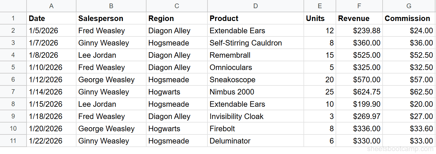
We’ll use a sales records table with 10 transactions. The Product column (D) has one duplicate: “Listening Device” appears in rows 2 and 8. All other product names are unique.

Sample Data

	A	B	C	D	E	F	G
1	Date	Salesperson	Region	Product	Units	Revenue	Commission
2	1/5/2026	Sherlock Holmes	Baker Street	Listening Device	12	$239.88	$24.00
3	1/7/2026	Irene Adler	Scotland Yard	Forensic Chemistry Set	8	$360.00	$36.00
4	1/8/2026	Inspector Lestrade	Baker Street	Pocket Watch	15	$525.00	$52.50
5	1/10/2026	Sherlock Holmes	Baker Street	Field Binoculars	5	$325.00	$32.50
6	1/12/2026	Mycroft Holmes	Scotland Yard	Cipher Decoder	20	$570.00	$57.00
7	1/14/2026	Irene Adler	Whitehall	Magnifying Glass	25	$624.75	$62.50
8	1/15/2026	Inspector Lestrade	Scotland Yard	Listening Device	10	$199.90	$20.00
9	1/18/2026	Sherlock Holmes	Baker Street	Disguise Kit	3	$269.97	$27.00
10	1/20/2026	Mycroft Holmes	Whitehall	Brass Telescope	8	$336.00	$33.60
11	1/22/2026	Irene Adler	Scotland Yard	Lockpick Set	6	$330.00	$33.00

Select the Product column

Highlight cells D2 through D11.

Open conditional formatting

Go to Format > Conditional formatting. Verify the “Apply to range” shows D2:D11.

Enter the COUNTIF formula

Select Custom formula is from the dropdown and enter:

Formula

=COUNTIF($D$2:$D$11, D2)>1

Set the highlight color and apply

Choose an orange fill color and click Done.

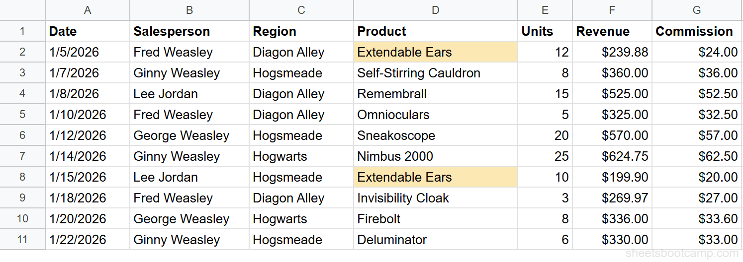
Two cells are highlighted: “Listening Device” in row 2 and “Listening Device” in row 8. Every other product name appears only once, so COUNTIF returns 1 and the formula returns FALSE for those cells.

Highlight Duplicates in the Salesperson Column

Apply the same pattern to B2:B11:

Formula

=COUNTIF($B$2:$B$11, B2)>1

In this dataset, every salesperson appears multiple times, Sherlock Holmes (rows 2, 5, 9), Irene Adler (rows 3, 7, 11), Inspector Lestrade (rows 4, 8), and Mycroft Holmes (rows 6, 10). Every cell is highlighted because no salesperson name is unique.

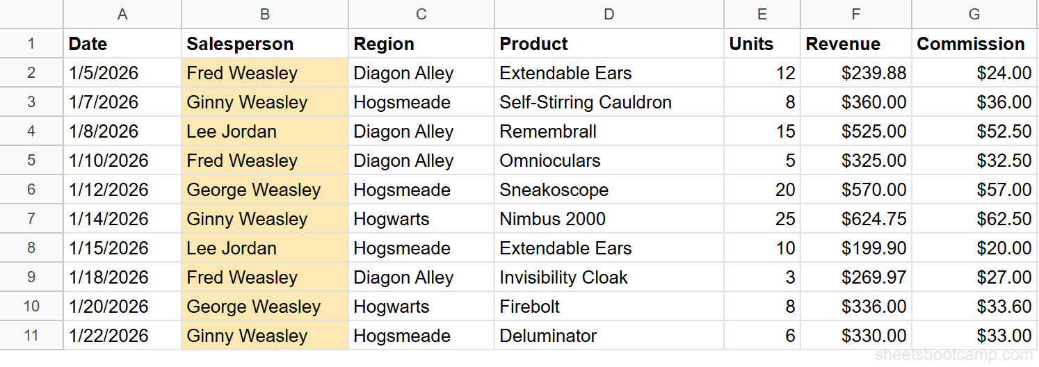
This demonstrates an important point: the formula highlights all occurrences of a duplicate, not the “extra” ones. If a name appears three times, all three cells are highlighted.

Tip

If every cell lights up, the column likely has no unique values. This is normal for category-like columns (regions, salesperson names, departments). Duplicate detection is most useful on columns where values should be unique, like order IDs, email addresses, or product SKUs.

Highlight Only the Second Occurrence

Sometimes you want to keep the first occurrence and flag only the repeat entries. Use a growing range:

Formula

=COUNTIF($D$2:D2, D2)>1

The difference is subtle but important. The range $D$2:D2 starts at D2 and ends at the current row. As the formula moves down:

Row	Range Evaluated	”Listening Device” Count	Highlighted?
2	D2:D2	1	No
3	D2:D3	0	No
8	D2:D8	2	Yes

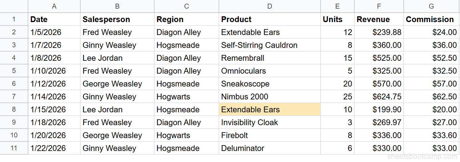
For row 2, the range is D2:D2, “Listening Device” appears once, so the count is 1 (not >1). For row 8, the range is D2:D8, “Listening Device” has already appeared in row 2, so the count is 2 (>1). Only the second occurrence gets highlighted.

Important

The growing range technique ($D$2:D2) only works when the end of the range is relative. If you accidentally write $D$2:$D$2, the range never grows and no duplicates are found.

Highlight Entire Rows with Duplicates

To color the entire row when a duplicate exists in the Product column, apply the rule to A2:G11 and lock the column reference:

Formula

=COUNTIF($D$2:$D$11, $D2)>1

Note the extra $ on $D2, this locks the column to D so that every cell in the row checks the same Product value. Without it, cell A2 would check D2 (correct), but cell E2 would check H2 (wrong).

Rows 2 and 8 are highlighted across all seven columns because both contain “Listening Device.”

For a detailed walkthrough of the entire-row technique, see conditional formatting entire row.

Common Mistakes

Forgetting absolute references on the COUNTIF range

If you write =COUNTIF(D2:D11, D2)>1, the range shifts as the formula moves down. For row 5, it evaluates D5:D14, three rows past your data. Always lock the range: $D$2:$D$11.

Using `=1` instead of `>1`

=COUNTIF($D$2:$D$11, D2)=1 highlights unique values, not duplicates. A value that appears once returns a count of 1 (TRUE). A value that appears twice returns 2 (FALSE). Use >1 to catch duplicates.

Applying to the wrong column

If you select B2:B11 (Salesperson) but the formula references column D (Product), the formula checks products but the formatting appears on salesperson names. Make sure the formula column matches the selected range, or use the $ technique for formatting based on another cell.

Warning

COUNTIF counts cells that match, including the cell itself. A value that appears exactly twice has a COUNTIF result of 2 in both cells. There is no built-in way to highlight “only the duplicate” without also highlighting the original, use the growing range technique for that.

Tips

Tip

Combine with Remove Duplicates. After identifying duplicates with conditional formatting, use Data > Data cleanup > Remove duplicates to delete the extra rows. Conditional formatting helps you verify which rows will be affected before removing them.

Check for near-duplicates. COUNTIF matches exact values only. “Listening Device” and “Listening Device ” (trailing space) are different. Use TRIM on your data first if extra spaces might cause mismatches.

Use COUNTIFS for multi-column duplicates. To find rows where both Salesperson AND Product match, use =COUNTIFS($B$2:$B$11, $B2, $D$2:$D$11, $D2)>1. This checks two columns at once and only highlights rows where the combination is duplicated.

Conditional Formatting: Complete Guide: all rule types, color scales, and managing multiple rules
Custom Formula in Conditional Formatting: write advanced rules with any formula that returns TRUE or FALSE
Conditional Formatting Entire Row: highlight all columns in a row based on one cell’s value
COUNTIF and COUNTIFS: the full COUNTIF function reference with counting patterns beyond duplicates

Highlight Duplicates in Google Sheets (Easy Guide)

In This Guide

The COUNTIF Formula for Duplicates