Custom Formula in Conditional Formatting (Google Sheets)
Learn how to write custom formula rules for conditional formatting in Google Sheets. Covers relative references, AVERAGE, LARGE, COUNTIF, and date patterns.
Sheets Bootcamp
March 5, 2026
Custom formula rules in conditional formatting let you use any Google Sheets formula to control formatting. Instead of picking from preset options like “Greater than” or “Text contains,” you write a formula that returns TRUE or FALSE. This is the most flexible rule type — anything you can calculate in a cell, you can use as a formatting condition.
This guide covers how custom formulas work, the critical role of relative and absolute references, and five ready-to-use formula patterns for common tasks.
In This Guide
- How Custom Formula Rules Work
- Step-by-Step: Highlight Above Average
- Relative vs. Absolute References
- Formula Patterns for Common Tasks
- Combining Multiple Functions
- Common Mistakes
- Tips
- Related Google Sheets Tutorials
- FAQ
How Custom Formula Rules Work
When you select Custom formula is as the rule type, you enter a formula in the value field. Google Sheets evaluates that formula for every cell in the “Apply to range.”
The formula is written relative to the first cell in the range. If your range is F2:F11, write the formula as if you are in cell F2. Sheets then adjusts the references for each subsequent cell — F3, F4, F5, and so on — following the same relative/absolute rules as regular formulas.
If the formula returns TRUE for a cell, that cell gets the formatting. If it returns FALSE, the cell stays unchanged.
The formula must return TRUE or FALSE (or a value that Sheets interprets as truthy/falsy). A formula that returns a number, text, or an error will not trigger formatting.
Step-by-Step: Highlight Above Average
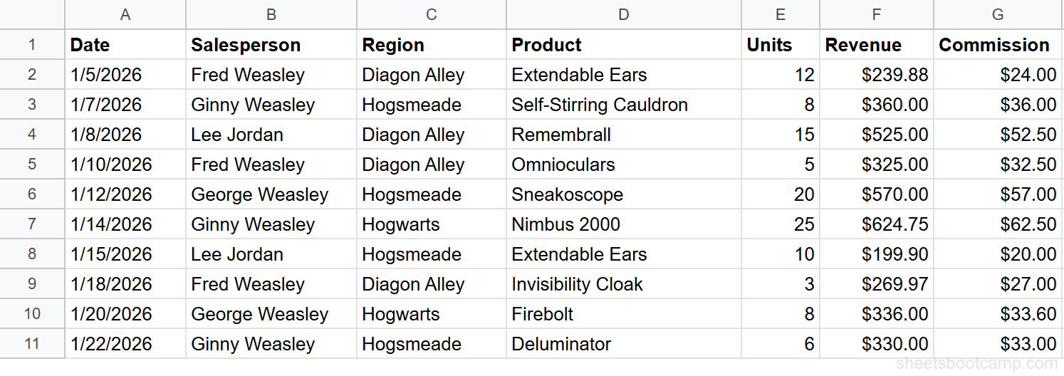
We’ll use a sales records table with 10 transactions. The goal: highlight Revenue cells that exceed the column average.
Sample Data
| A | B | C | D | E | F | G | |
|---|---|---|---|---|---|---|---|
| 1 | Date | Salesperson | Region | Product | Units | Revenue | Commission |
| 2 | 1/5/2026 | Fred Weasley | Diagon Alley | Extendable Ears | 12 | $239.88 | $24.00 |
| 3 | 1/7/2026 | Ginny Weasley | Hogsmeade | Self-Stirring Cauldron | 8 | $360.00 | $36.00 |
| 4 | 1/8/2026 | Lee Jordan | Diagon Alley | Remembrall | 15 | $525.00 | $52.50 |
| 5 | 1/10/2026 | Fred Weasley | Diagon Alley | Omnioculars | 5 | $325.00 | $32.50 |
| 6 | 1/12/2026 | George Weasley | Hogsmeade | Sneakoscope | 20 | $570.00 | $57.00 |
| 7 | 1/14/2026 | Ginny Weasley | Hogwarts | Nimbus 2000 | 25 | $624.75 | $62.50 |
| 8 | 1/15/2026 | Lee Jordan | Hogsmeade | Extendable Ears | 10 | $199.90 | $20.00 |
| 9 | 1/18/2026 | Fred Weasley | Diagon Alley | Invisibility Cloak | 3 | $269.97 | $27.00 |
| 10 | 1/20/2026 | George Weasley | Hogwarts | Firebolt | 8 | $336.00 | $33.60 |
| 11 | 1/22/2026 | Ginny Weasley | Hogsmeade | Deluminator | 6 | $330.00 | $33.00 |
Select the range to format
Highlight cells F2 through F11 — the Revenue column.
Enter the custom formula
Go to Format > Conditional formatting. Select Custom formula is from the dropdown and enter:
=F2>AVERAGE($F$2:$F$11)The F2 is relative — it adjusts for each row (F3, F4, etc.). The $F$2:$F$11 is absolute — it stays fixed so the AVERAGE always covers the full column.
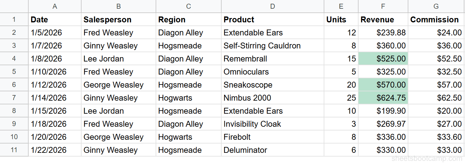
The average of the 10 revenue values is $378.05.
Choose formatting and review
Pick a green fill color and click Done. Three cells are highlighted: $525.00 (row 4), $570.00 (row 6), and $624.75 (row 7). These are the only values above the $378.05 average.
Relative vs. Absolute References
This is the most important concept for custom formula rules. The dollar sign ($) controls which parts of a reference stay fixed and which parts shift.
| Reference | Column | Row | When to Use |
|---|---|---|---|
$C2 | Locked | Shifts | Check one column across all rows (e.g., Region = “Hogwarts”) |
C$2 | Shifts | Locked | Compare against a fixed row (rare in CF) |
$C$2 | Locked | Locked | Reference a single fixed cell (e.g., a threshold in I1) |
C2 | Shifts | Shifts | Let everything shift (standard for single-column rules on the same column) |
The Rule of Thumb
- Formatting one column based on itself (F2:F11, checking revenue): Use
F2— no dollar signs needed because the formula stays in the same column. - Formatting based on another column (format F based on C): Use
$C2— lock the column, let the row shift. - Referencing a fixed cell (threshold in I1): Use
$I$1— lock everything. - Formatting entire rows (A2:G11): Use
=$C2— lock the column so every cell in the row checks the same column.
When in doubt, test the formula in a regular cell first. Enter it in F2 and drag down to see if it returns TRUE for the correct rows. If it works there, it will work in conditional formatting.
Formula Patterns for Common Tasks
Pattern 1: Above or Below Average
Highlight cells above the average:
=F2>AVERAGE($F$2:$F$11)Highlight cells below the average:
=F2<AVERAGE($F$2:$F$11)The AVERAGE range uses absolute references so it stays fixed. The cell reference (F2) is relative so it shifts per row.
Pattern 2: Top N Values
Highlight the top 3 revenue values:
=F2>=LARGE($F$2:$F$11, 3)LARGE returns the 3rd-largest value ($525.00). Any cell greater than or equal to that is highlighted. Result: $525.00, $570.00, $624.75.
To highlight the bottom 3, use SMALL:
=F2<=SMALL($F$2:$F$11, 3)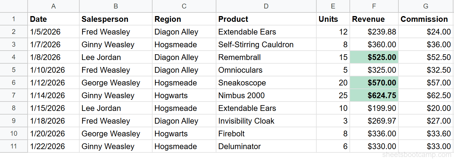
Pattern 3: Highlight Rows by Text Match
Applied to A2:G11 to color entire rows where Region is “Hogwarts”:
=$C2="Hogwarts"The $C locks to the Region column. Every cell in the row evaluates the same formula, so the entire row lights up. See highlighting entire rows for a detailed walkthrough.
Pattern 4: Highlight Blank or Non-Blank Cells
Highlight empty cells:
=ISBLANK(A2)Highlight cells with content:
=NOT(ISBLANK(A2))ISBLANK returns TRUE for genuinely empty cells. Cells with spaces or zero-length strings may not trigger — use =LEN(TRIM(A2))=0 as an alternative that catches invisible whitespace.
Pattern 5: Date Comparisons
Highlight dates older than 30 days from today:
=A2<TODAY()-30Highlight dates in the current month:
=AND(MONTH(A2)=MONTH(TODAY()), YEAR(A2)=YEAR(TODAY()))TODAY() updates automatically, so the formatting adjusts each day without editing the rule. For more date-based patterns, see conditional formatting with dates.
Combining Multiple Functions
You can use AND, OR, and nested functions to create precise conditions.
AND: Both Conditions Must Be True
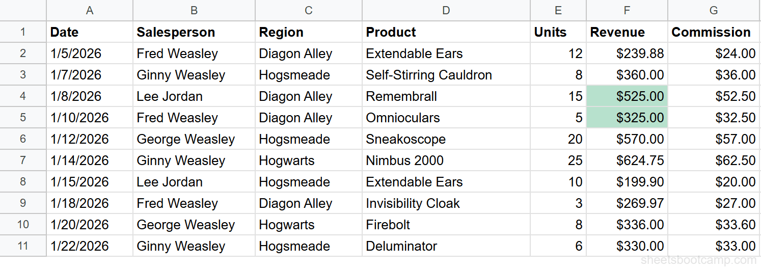
Highlight Revenue cells where the region is “Diagon Alley” AND revenue exceeds $300. Apply to F2:F11:
=AND($C2="Diagon Alley", F2>300)Two cells match: Lee Jordan’s $525.00 (row 4) and Fred Weasley’s $325.00 (row 5). Both are Diagon Alley transactions with revenue above $300.
OR: Either Condition Can Be True
Highlight Revenue cells from either Hogwarts or Hogsmeade. Apply to F2:F11:
=OR($C2="Hogwarts", $C2="Hogsmeade")Six cells match — all transactions from those two regions.
Nested Logic
Highlight cells where revenue is above average AND the salesperson name contains “Weasley”:
=AND(F2>AVERAGE($F$2:$F$11), ISNUMBER(SEARCH("Weasley", $B2)))Two cells match: George Weasley’s $570.00 (row 6) and Ginny Weasley’s $624.75 (row 7). Lee Jordan’s $525.00 is above average but excluded because the name does not contain “Weasley.”
SEARCH is case-insensitive. If you need case-sensitive matching, use FIND instead of SEARCH.
Common Mistakes
Formula does not start with =
The formula field requires an equals sign at the beginning. Without it, Sheets treats the text as a literal string comparison and the rule never triggers.
Wrong reference style
If your range is F2:F11 and your formula references F1, the formula is off by one row. The formula should reference the first row of the “Apply to range” — in this case, row 2.
Selected the wrong rule type
If you enter =F2>400 but the dropdown says “Text contains” instead of “Custom formula is,” Sheets looks for cells containing the literal text =F2>400. The formula never evaluates. Always verify the dropdown says Custom formula is.
Formula returns a value instead of TRUE/FALSE
A formula like =F2-400 returns a number (like 125), not TRUE or FALSE. Sheets may interpret positive numbers as truthy, but the behavior is unreliable. Write the formula as an explicit comparison: =F2-400>0 or =F2>400.
If your formula references a cell in a different sheet (like =Sheet2!A1), it might not evaluate correctly in conditional formatting. Custom formula rules work best when referencing cells on the same sheet as the formatted range.
Tips
Build formulas incrementally. Start with a basic condition that works, then add complexity. Get =F2>400 working first, then expand to =AND(F2>400, $C2="Diagon Alley").
Copy the formula from a cell. Enter the formula in an empty cell, verify it returns TRUE/FALSE for the correct rows, then copy and paste it into the conditional formatting rule. This avoids typos in the small input field.
Use named ranges for readability. If you use the same AVERAGE range in multiple rules, define a named range (Data > Named ranges). Then write =F2>AVERAGE(RevenueRange) instead of =F2>AVERAGE($F$2:$F$11).
Related Google Sheets Tutorials
- Conditional Formatting: Complete Guide — covers all rule types, color scales, and managing multiple rules
- Format Based on Another Cell — highlight cells in one column based on values in another column
- Conditional Formatting Entire Row — apply formatting across all columns based on one cell’s value
- Highlight Duplicates — find and color duplicate values using COUNTIF in custom formulas
- IF Function: Complete Guide — logical tests in formulas, the same AND/OR patterns used in custom formatting rules
Frequently Asked Questions
How do I use a custom formula in conditional formatting?
Select the range to format, go to Format > Conditional formatting, and choose “Custom formula is” from the dropdown. Enter any formula that returns TRUE or FALSE. The formula is evaluated relative to the first cell in the range, and references shift row by row. For example, =F2>400 applied to F2:F11 highlights cells above 400.
What does Custom formula is mean in Google Sheets conditional formatting?
“Custom formula is” lets you write your own rule instead of picking from built-in options like “Greater than” or “Text contains.” You enter a formula that returns TRUE or FALSE. Cells where the formula returns TRUE get the formatting. This gives you access to any Google Sheets function — AVERAGE, COUNTIF, TODAY, AND, OR — in your formatting logic.
Why is my custom formula conditional formatting not working?
Check four things. First, the formula starts with an equals sign (=). Second, you selected “Custom formula is” from the dropdown, not another rule type. Third, the formula references the correct first row of your range (row 2 if your range starts at row 2). Fourth, your dollar signs are correct — lock columns that should stay fixed with $. Test the formula in a regular cell to confirm it returns TRUE and FALSE for the expected rows.
Can I use functions like AVERAGE, COUNTIF, or TODAY in conditional formatting?
Yes. Any function that produces a result you can compare to TRUE or FALSE works inside a custom formula rule. For example, =F2>AVERAGE($F$2:$F$11) highlights cells above the average, =COUNTIF($B$2:$B$11, B2)>1 highlights duplicates, and =A2<TODAY()-30 highlights dates older than 30 days.
How do I apply a custom formula rule to an entire row?
Select the full row range (like A2:G11) and enter a formula with a locked column reference. For example, =$C2="Hogwarts" checks column C for every row and formats all columns in matching rows. The $ on the column is essential — without it, the column reference shifts and checks the wrong data. See the full walkthrough in our entire row formatting guide.