Data Validation in Google Sheets: Complete Guide
Learn how to use data validation in Google Sheets to create dropdown lists, restrict input, add checkboxes, and write custom rules. Step-by-step guide.
Sheets Bootcamp
February 18, 2026
Data validation in Google Sheets controls what users can enter in a cell. You define rules — a list of allowed values, a date range, a number threshold, or a custom formula — and Sheets enforces them. Any entry that breaks a rule gets rejected or flagged.
This guide covers how to set up validation rules, create dropdown lists, add checkboxes, restrict dates, write custom formula rules, and configure error messages. We’ll use a Hogwarts task tracker with 10 rows as the working example.
In This Guide
- What Is Data Validation?
- How to Add Data Validation: Step-by-Step
- Validation Rule Types
- Practical Examples
- Custom Error Messages
- Common Mistakes and Fixes
- Tips and Best Practices
- Related Google Sheets Tutorials
- FAQ
What Is Data Validation?
Data validation restricts what can be entered in a cell. Instead of trusting every collaborator to type the right value, you define rules that Sheets enforces automatically. A cell with a dropdown only accepts the options you listed. A cell with date validation rejects text. A cell with a custom formula rule blocks entries that fail your condition.
This matters because bad data is quiet. Someone types “Hgih” instead of “High” in a priority column, and every formula that checks for “High” misses that row. A COUNTIF that counts “Complete” tasks returns the wrong number because one cell says “Done” instead. Data validation catches these mistakes at the point of entry, before they spread through your formulas.
Common uses include:
- Dropdown lists for categories like status, priority, or department
- Checkboxes for yes/no fields like task completion
- Date restrictions to prevent past or future dates
- Number ranges to limit values (e.g., quantities between 1 and 100)
- Custom formulas for any rule you can express as TRUE or FALSE
You define each rule once, and it applies to every cell in the range. When new rows get added, copy the validation down to include them.
How to Add Data Validation: Step-by-Step
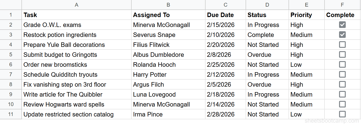
We’ll use a task tracker with 10 tasks assigned to Hogwarts staff. The goal: create a dropdown list in the Status column (D2:D11) with four allowed values — Not Started, In Progress, Complete, and Overdue.
Sample Data
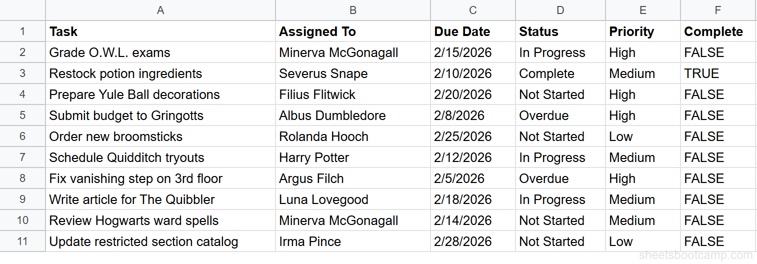
The table has six columns: Task (A), Assigned To (B), Due Date (C), Status (D), Priority (E), and Complete (F). Status currently has free-text values — we’ll replace those with a controlled dropdown.
Select the cells to validate
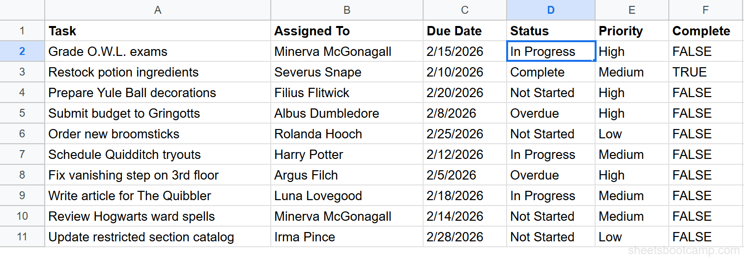
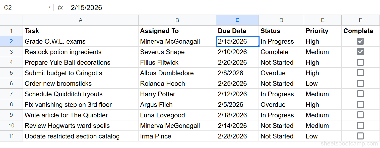
Highlight cells D2 through D11 — the Status column, excluding the header. The range you select determines which cells the rule applies to.
Open Data validation
Go to Data > Data validation in the menu bar. The data validation panel opens on the right side of the screen. The “Apply to range” field should show D2:D11. If it shows a single cell, you can type the full range manually.
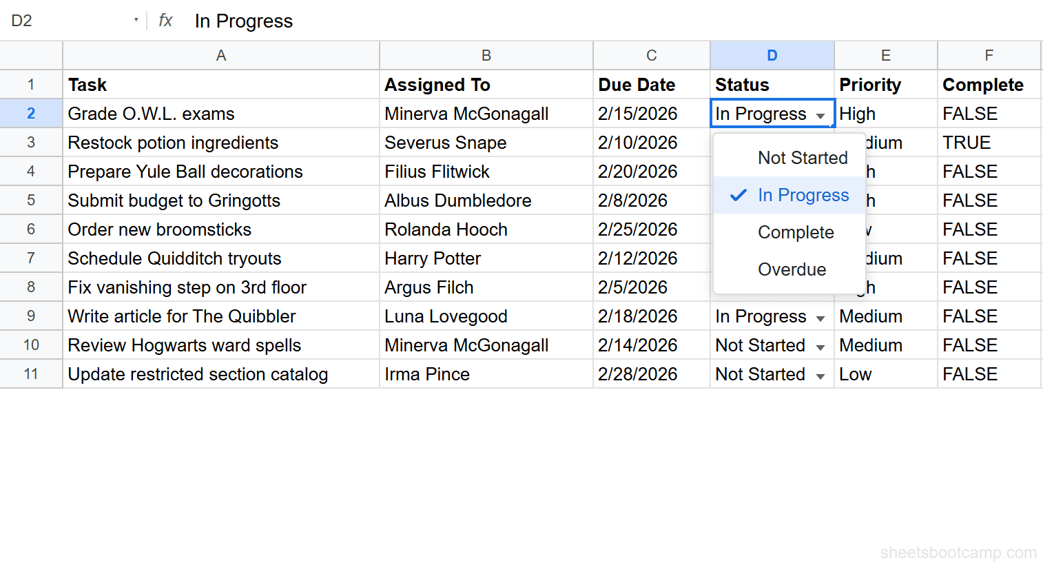
Set criteria to Dropdown and enter values
Under Criteria, select Dropdown from the list. Enter four values, one per line: Not Started, In Progress, Complete, and Overdue. Google Sheets assigns a color chip to each option by default — you can customize these or leave them as-is.
Set invalid data handling to Reject input
Scroll down in the validation panel. Under If the data is invalid, choose Reject input. This blocks any value that doesn’t match one of the four dropdown options. The alternative, “Show warning,” allows the entry but marks it with an orange triangle.
Test the dropdown
Click any cell in D2:D11. A dropdown arrow appears on the right edge of the cell. Click it to see the four options. Select one to update the value. Now try typing “Pending” directly into a cell — Sheets rejects it with an error message because “Pending” is not in the list.
To edit a validation rule later, select any cell in the range and go to Data > Data validation. The existing rule appears in the panel. You can change the criteria, add options, or switch between “Reject input” and “Show warning” at any time.
Validation Rule Types
Google Sheets offers several criteria types for data validation. Each one restricts input differently.
| Rule Type | What It Does | Example Use Case |
|---|---|---|
| Dropdown | Limits input to a predefined list of values | Status column: Not Started, In Progress, Complete, Overdue |
| Dropdown (from a range) | Pulls list items from a cell range | Department list sourced from a reference sheet |
| Checkbox | Inserts a clickable checkbox (TRUE/FALSE) | Task completion toggle |
| Number | Restricts to numeric values with conditions (between, greater than, etc.) | Budget amounts between 0 and 10,000 |
| Text | Validates text content (contains, is valid email, is valid URL) | Email address column |
| Date | Restricts to valid dates with optional conditions (before, after, between) | Due dates that must be in the future |
| Custom formula is | Accepts any formula returning TRUE or FALSE | =C2>=TODAY() to block past due dates |
The Dropdown and Checkbox types are the most commonly used. Custom formula is the most flexible — it can enforce any rule you can express as a formula.
Practical Examples
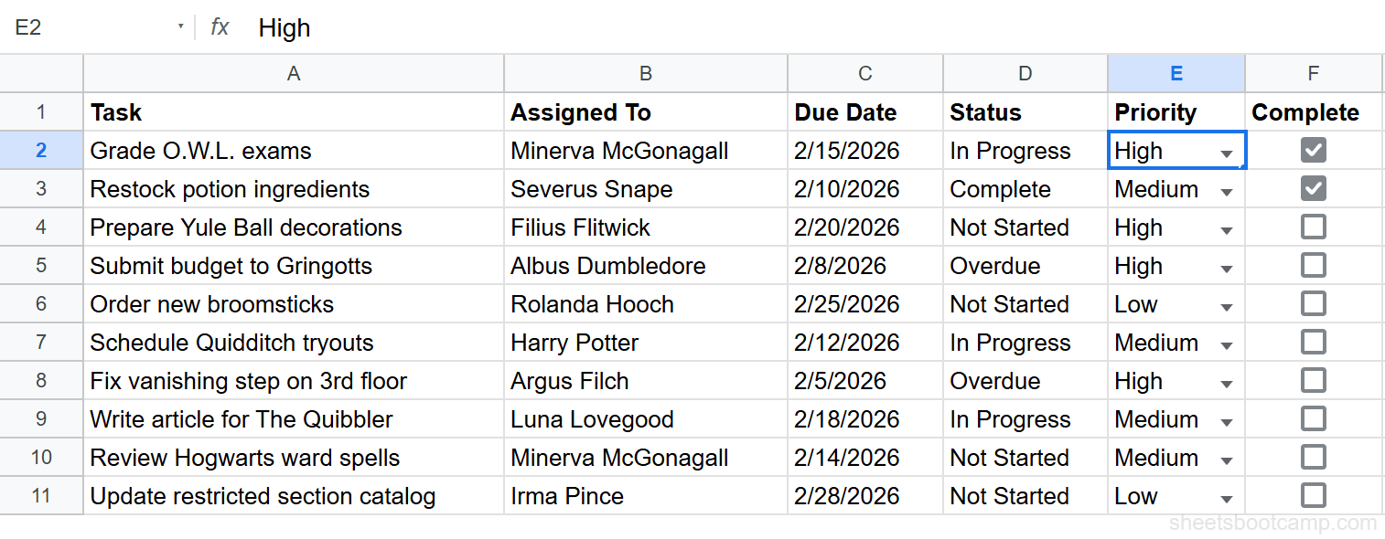
Example 1: Priority Dropdown
The Priority column (E2:E11) should accept only three values: High, Medium, and Low. The setup is identical to the Status dropdown from the step-by-step section.
- Select E2:E11
- Go to Data > Data validation
- Choose Dropdown and enter:
High,Medium,Low - Set to Reject input
Every cell in the column now shows a dropdown arrow. Formulas like =COUNTIF(E2:E11, "High") return accurate counts because the only possible values are the three you defined. No typos, no variations.
For a detailed walkthrough of dropdown features including multi-select and dynamic lists, see creating dropdown lists in Google Sheets.
Example 2: Checkboxes for Task Completion
The Complete column (F2:F11) tracks whether each task is done. Instead of typing TRUE or FALSE, a checkbox gives collaborators a single click to toggle the value.
- Select F2:F11
- Go to Data > Data validation
- Choose Checkbox as the criteria
- Click Done
Each cell displays a clickable checkbox. Checked = TRUE, unchecked = FALSE. These Boolean values work in formulas. To count completed tasks, use =COUNTIF(F2:F11, TRUE). To count remaining tasks, use =COUNTIF(F2:F11, FALSE).
You can also combine checkboxes with other functions. =SUMPRODUCT((F2:F11=FALSE)*(E2:E11="High")) returns the number of incomplete high-priority tasks — useful for tracking what needs attention. For more on combining TRUE/FALSE logic with formulas, see the IF function guide.
For more on checkbox formulas and conditional formatting with checkboxes, see checkboxes in Google Sheets.
Example 3: Date Validation
The Due Date column (C2:C11) should accept only valid dates. You can also restrict dates to a range — for example, only dates within the current quarter.
- Select C2:C11
- Go to Data > Data validation
- Choose Date > is valid date as the criteria
- Set to Reject input
With “is valid date” selected, Sheets rejects any text that isn’t a recognizable date. Typing “next Tuesday” or “asap” triggers an error. For stricter control, use “is after” with a specific date to prevent past dates, or “is between” to limit to a date range.
Google Sheets dates are numbers with date formatting applied. The “is valid date” rule checks whether the cell value can be interpreted as a date — not whether the date makes sense for your project. For business logic like “due date must be in the future,” use a custom formula rule instead.
For date range validation patterns and dynamic date rules, see date validation in Google Sheets.
Example 4: Custom Formula — No Past Due Dates
A custom formula rule can enforce any condition. Here, we’ll prevent users from entering due dates that have already passed.
- Select C2:C11
- Go to Data > Data validation
- Choose Custom formula is
- Enter the formula:
=C2>=TODAY()This formula compares each cell in the Due Date column against today’s date. If the entered date is today or later, the formula returns TRUE and the entry is accepted. If the date is in the past, it returns FALSE and Sheets rejects it (or shows a warning, depending on your setting).
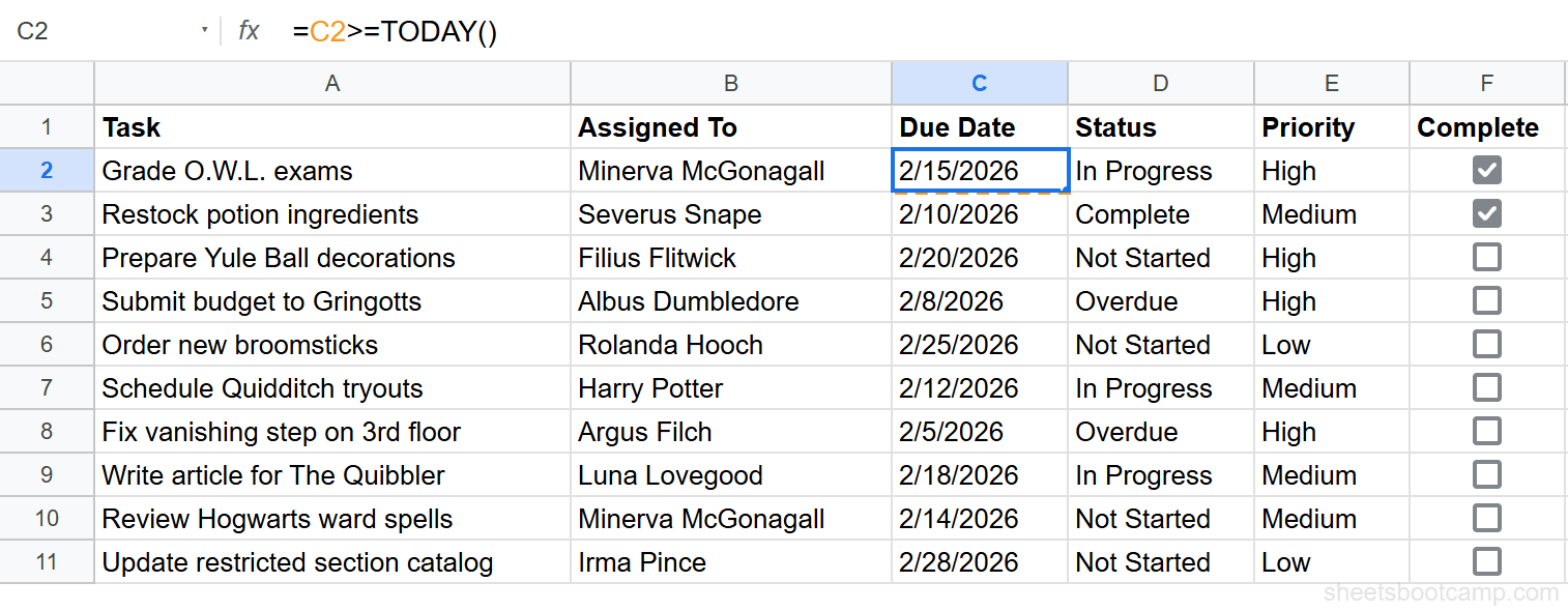
The formula uses a relative reference (C2) because it needs to shift for each row in the range. The TODAY function updates automatically, so the rule always compares against the current date.
Write the custom formula as if you’re in the first cell of the validation range. If your range starts at C2, the formula should reference C2. Sheets adjusts the reference for each subsequent row — C3, C4, C5, and so on.
Custom formulas open up validation possibilities that built-in rules can’t handle: cross-column checks, text pattern matching, and calculations involving multiple cells. For more patterns, see data validation with custom formulas.
Custom Error Messages
When someone enters invalid data, Google Sheets can respond in two ways.
Reject Input vs. Show Warning
Reject input blocks the entry entirely. The cell reverts to its previous value, and an error dialog appears. The user must enter a valid value or cancel.
Show warning accepts the entry but marks the cell with a small orange triangle in the upper-right corner. Hovering over the triangle displays the warning message. The invalid data stays in the cell.
Use “Reject input” for columns where accuracy is non-negotiable — status codes, IDs, and any field that feeds into formulas. Use “Show warning” for columns where flexibility matters more than enforcement, like freeform notes with a suggested format.
Adding Help Text
You can add a custom message that appears when a user selects a validated cell. In the data validation panel, expand the Advanced options section and enable “Show validation help text.” Enter a message like “Choose a status: Not Started, In Progress, Complete, or Overdue.”
This help text appears as a small tooltip below the cell. It guides collaborators who don’t know the allowed values, reducing errors before they happen.
Example: Rejection in Action
If someone types “Pending” into a cell validated with the Status dropdown and “Reject input” enabled, Sheets blocks the entry and shows an error.
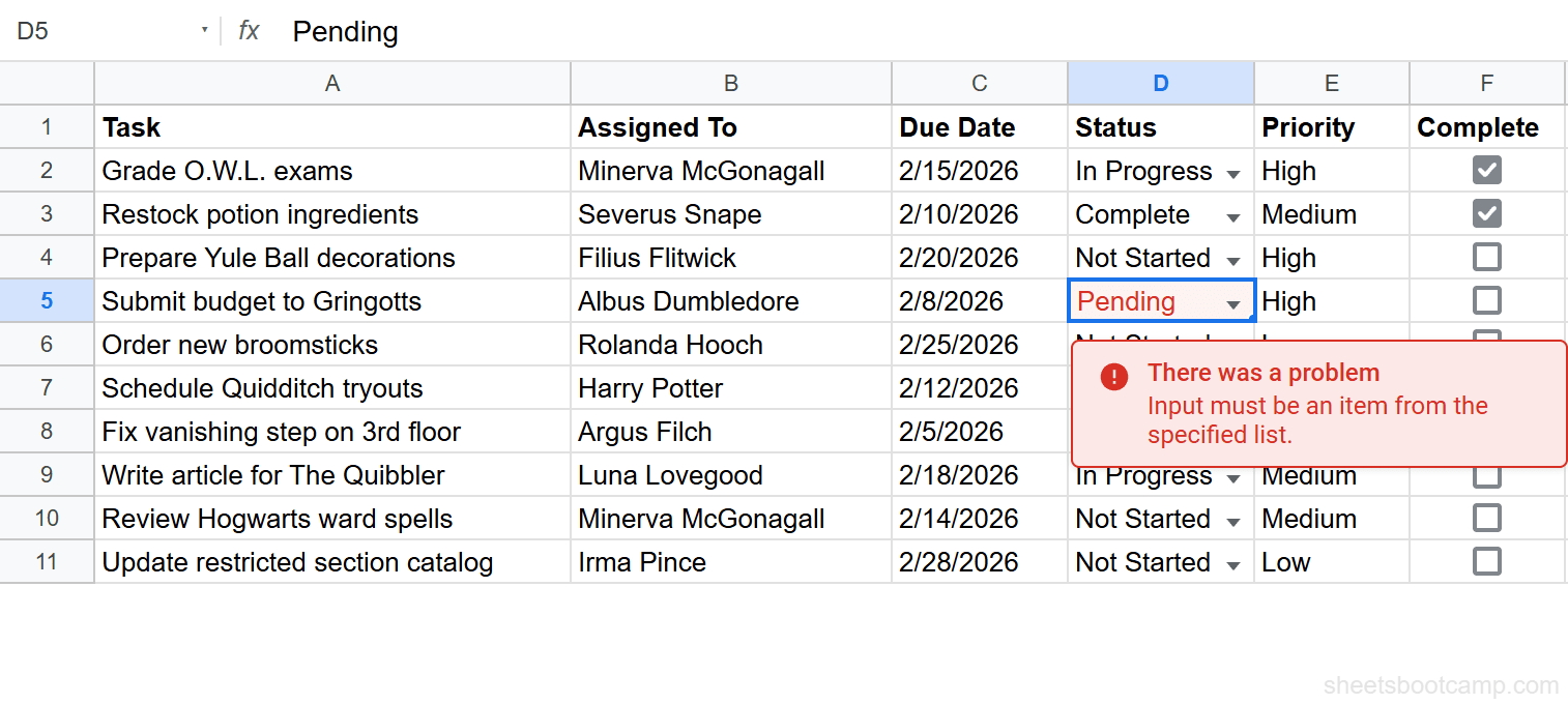
The cell keeps its previous value. The user must pick from the dropdown or enter one of the four allowed values.
For detailed coverage of error message customization, see custom error messages for data validation.
Common Mistakes and Fixes
Validation Not Applied to the Whole Range
You set up a rule, but only some cells have the dropdown or restriction. This happens when you select a single cell or a partial range before opening Data validation.
Fix: Open the rule, check the “Apply to range” field, and expand it to cover the full range (e.g., D2:D11 instead of D2:D5). You can also select the full range first, then open Data > Data validation.
”Show Warning” When You Meant “Reject Input”
Invalid data is getting through. The cells have orange triangles, but the bad values are still there. This means the rule is set to “Show warning” instead of “Reject input.”
Fix: Open Data > Data validation, find the rule, and change the invalid data handling to “Reject input.” Existing invalid values won’t be removed automatically — you’ll need to correct those manually.
Dropdown Items with Extra Spaces
Your dropdown shows “High” and ” High” as separate options, or formulas checking for “High” miss cells that look correct. Invisible leading or trailing spaces in the dropdown values cause this.
Fix: Open the validation rule and retype each dropdown option. Check for spaces before and after each value. In the validated cells, use =TRIM(D2) in a helper column to verify whether existing values have hidden spaces.
Custom Formula Reference Errors
Your custom formula validation doesn’t work — it either rejects everything or accepts everything. The formula references are wrong.
Fix: Make sure the formula references the first cell in the validation range. If the range is C2:C11, the formula should use C2, not C1 or $C$2. Use a relative row reference so the formula shifts for each row. Test the formula in a regular cell first to confirm it returns TRUE and FALSE for the expected rows.
Checkbox Column Showing TRUE/FALSE Text
The Complete column shows the words TRUE and FALSE instead of checkboxes. This happens when the checkbox validation was removed or never applied, but the cell values remain.
Fix: Select the range, go to Data > Data validation, and apply the Checkbox criteria. The TRUE/FALSE text values convert to checked/unchecked checkboxes. If the column contains other values like “Yes” or “No,” you’ll need to convert them to TRUE/FALSE first.
Pasting data into validated cells can bypass validation rules. If you paste from an external source, Sheets accepts the pasted values even if they violate the rule. After pasting, verify the data or re-apply the validation rule to catch any invalid entries.
Tips and Best Practices
-
Combine data validation with conditional formatting. Validation prevents bad data from entering a cell. Conditional formatting highlights problems visually. Use both: a dropdown for the Status column plus a conditional formatting rule that turns “Overdue” cells red.
-
Use “Reject input” for columns that feed into formulas. If a COUNTIF counts “Complete” tasks, one cell with “Completed” (extra “d”) breaks the count. “Reject input” ensures every value matches exactly.
-
Add help text for shared spreadsheets. Collaborators who didn’t build the sheet won’t know the allowed values. A help text tooltip like “Enter a date in the future” saves back-and-forth messages.
-
Use a hidden sheet for long dropdown lists. Instead of typing 50 department names into the validation criteria, list them on a separate “Reference” sheet and use “Dropdown (from a range)” pointing to that list. Updating the reference sheet updates every dropdown in the workbook. You can even use VLOOKUP to cross-reference validated entries against a lookup table on that reference sheet.
-
Apply validation before sharing the spreadsheet. Set up all rules while you have full control. Once collaborators start entering data, fixing validation gaps means cleaning up existing bad entries.
-
Test validation rules after setup. Enter a valid value and an invalid value in each validated column. Confirm the valid entry is accepted and the invalid entry is rejected (or warned). A rule that looks correct in the panel can still behave unexpectedly if the range or formula reference is off.
Related Google Sheets Tutorials
- Create Dropdown Lists in Google Sheets — Build single-select and multi-option dropdowns with color coding
- Dependent Dropdown Lists — Create cascading dropdowns where the second list changes based on the first selection
- Data Validation with Custom Formulas — Write advanced validation rules using any formula that returns TRUE or FALSE
- Date Validation in Google Sheets — Restrict date entry to valid dates, future dates, or specific date ranges
- Checkboxes in Google Sheets — Insert checkboxes and use them in COUNTIF, SUMPRODUCT, and IF formulas
- Custom Error Messages for Data Validation — Configure rejection messages, warnings, and input help text
- Conditional Formatting in Google Sheets — Highlight cells by value, color-code data, and build formula-based formatting rules
- IF Function in Google Sheets — Use IF for logical tests in formulas, a natural companion to custom validation rules
- VLOOKUP in Google Sheets — Look up values across tables, useful when validating entries against a reference list
- QUERY Function in Google Sheets — Filter and aggregate data with SQL-like syntax, useful for building validation source ranges
Frequently Asked Questions
How do I create a dropdown list in Google Sheets?
Select the cells, go to Data > Data validation, set the criteria to “Dropdown,” and enter your list items separated by commas. Each cell in the range gets a dropdown arrow that shows your options when clicked. You can also source the list from a cell range using “Dropdown (from a range)” for longer or frequently changing lists.
How do I add a checkbox in Google Sheets?
Select the cells, go to Data > Data validation, and choose “Checkbox” as the criteria. Checkboxes store TRUE when checked and FALSE when unchecked, so you can use them in formulas like =COUNTIF(F2:F11, TRUE) to count checked items or =SUMPRODUCT for conditional calculations.
Can I use data validation with a custom formula?
Yes. Choose “Custom formula is” as the criteria and enter any formula that returns TRUE or FALSE. For example, =C2>=TODAY() prevents users from entering past dates. The formula is evaluated relative to the first cell in the range, and Sheets adjusts the reference for each subsequent row.
How do I remove data validation in Google Sheets?
Select the cells with validation, go to Data > Data validation, and click “Remove validation” at the bottom of the panel. This removes the rule but keeps any data already in the cells. To remove validation from multiple ranges, you’ll need to select each validated range and remove its rule individually.
What happens when someone enters invalid data?
It depends on the setting you chose. “Reject input” blocks the entry entirely and shows an error message — the cell reverts to its previous value. “Show warning” allows the entry but displays an orange triangle in the corner of the cell to flag it. Hovering over the triangle shows the warning text.
Can I apply data validation to multiple cells at once?
Yes. Select the entire range before opening Data > Data validation. The rule applies to every cell in the selection. You can also type a range like D2:D100 directly in the “Apply to range” field. For non-contiguous ranges, add multiple ranges separated by commas.
How do I create dependent dropdown lists?
Use INDIRECT in the data validation criteria to reference a named range that changes based on another cell’s value. Set up named ranges for each option set (e.g., “Marketing” and “Engineering” as range names), then set the dependent cell’s validation source to =INDIRECT(A2). When A2 changes, the dropdown options update. For the full walkthrough, see dependent dropdown lists in Google Sheets.
Does data validation work on mobile?
Yes, but with limitations. Dropdowns and checkboxes work in the Google Sheets mobile app — you can tap a cell and select from the list or toggle a checkbox. Custom formula validation and some advanced options are not available for editing on mobile. Set up validation rules on desktop for full access to all features.