Dependent Drop-Down Lists in Google Sheets

A dependent dropdown Google Sheets list changes its options based on what you selected in another dropdown. You’ll find this technique covered in the Google Sheets data validation guide as one of the more useful validation setups. If you haven’t built a basic dropdown yet, start with dropdown lists in Google Sheets before continuing here.

The technique connects two dropdowns using the INDIRECT function and named ranges. Select “Teaching” in the Department column and the Staff column shows only Teaching staff. Select “Administration” and the list updates automatically.

In This Guide

• What Are Dependent Dropdowns?
• Set Up the Source Data
• How to Create Dependent Dropdowns: Step-by-Step
• How INDIRECT Makes It Work
• Common Mistakes
• Tips
• Related Google Sheets Tutorials
• Frequently Asked Questions

What Are Dependent Dropdowns?

A dependent dropdown shows different options depending on what you chose in a previous dropdown. The second list is linked to the first.

Real-world uses include:

• Country / State: Select United States and see US states. Select Canada and see Canadian provinces.
• Department / Employee: Select a department and see only the staff in that department.
• Category / Subcategory: Select “Hardware” and see hardware subcategories. Select “Software” and see software subcategories.

The result is a cleaner, more accurate data entry experience. Users can only select combinations that make sense.

Set Up the Source Data

Before you add any validation rules, you need a reference area that lists each option group. This reference data is what Google Sheets will pull from when it builds each dropdown.

Here is the layout for a Whitehall staff tracker:

• Column H: Department names (Teaching, Administration, Activities, Facilities)
• Column I: Teaching staff list
• Column J: Administration staff list
• Column K: Activities staff list

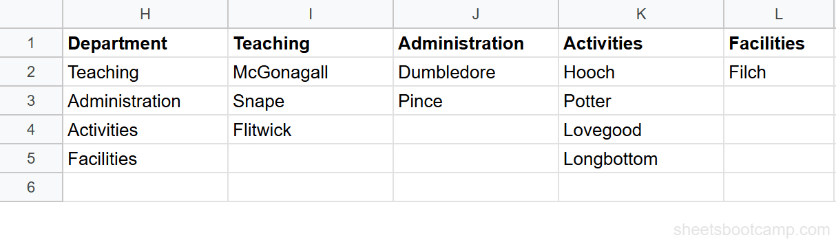
Each column holds the members for one department. You’ll turn each staff column into a named range in Step 3.

How to Create Dependent Dropdowns: Step-by-Step

Step 1: Create the Department Dropdown

Select the cell where users will choose a department. In this example, that’s G2.

Go to Data > Data validation > Add rule. Under Criteria, select Dropdown (from a range). Point it to the department names in H2:H5, or choose List of items and type the names directly: Teaching, Administration, Activities, Facilities.

Click Done. You now have a working Department dropdown in G2. The Staff column is still empty. You’ll connect it in Step 3.

Step 2: Create a Named Range for Each Department

A named range gives a cell range a name you can reference by text. This is the key to how INDIRECT works.

Select the Teaching staff list, I2:I4. Go to Data > Named ranges. In the panel that opens, type Teaching as the name and confirm the range is I2:I4. Click Done.

Repeat for each department:

Named Range	Range	Staff
Teaching	I2:I4	Hudson, Moran, Morstan
Administration	J2:J3	Holmes, Adler
Activities	K2:K5	Watson, Holmes, Morstan, Mortimer
Facilities	L2:L2	Barrymore

Step 3: Put INDIRECT in a Helper Cell

This is the step most guides get wrong. You cannot type =INDIRECT(G2) straight into the data validation range box: Google Sheets refuses it and shows “Please enter a valid range”. The validation box accepts a range, and INDIRECT is a formula.

So give the formula a cell of its own. Click a spare cell out of the way, such as N2, and enter:

Whatever list G2 names now spills down that column. With “Teaching” in G2, N2:N4 fills with Hudson, Moran, and Morstan.

Step 4: Point the Staff Dropdown at the Helper Range

Select the Staff cell, H2. Go to Data > Data validation > Add rule. Under Criteria, select Dropdown (from a range). In the Cell range box, enter the helper range:

Click Done. The dropdown now reads the helper column, and the helper follows G2.

Step 5: Test the Dropdowns

Select G2 and choose Teaching from the Department dropdown. Then select H2 and open the Staff dropdown. You should see Hudson, Moran, and Morstan.

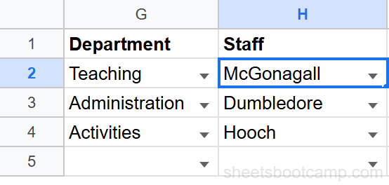
Now change G2 to Administration. Select H2 again and open the dropdown. The list now shows Holmes and Adler.

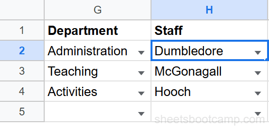
The Staff dropdown updates every time the Department selection changes. You don’t have to modify any validation rules.

How INDIRECT Makes It Work

INDIRECT converts a text string into a range reference. Google Sheets evaluates it at the moment the cell is used, not when you set up the formula.

When G2 contains “Teaching”, =INDIRECT(G2) in the helper cell is the same as =INDIRECT("Teaching"). Google Sheets looks for a named range called Teaching, finds I2:I4, and spills those names down the helper column.

When G2 changes to “Administration”, INDIRECT re-evaluates and the helper column re-spills to J2:J3, the Administration named range. The dropdown rule never changes: it always points at the same helper range, and the helper is what moves.

The formula never changes. What changes is the text value in G2, and that text controls which named range INDIRECT points to.

This is why the named range names must match the dropdown values exactly. INDIRECT is only as accurate as the text it receives.

Common Mistakes

Spaces in Department Names Break Named Ranges

Google Sheets named ranges cannot contain spaces. If your department is called “Customer Support”, you cannot create a named range named “Customer Support”. The name would be rejected.

You have two options:

1. Use underscores in both the dropdown value and the named range name: “Customer_Support”
2. Keep the readable label in the dropdown but use SUBSTITUTE in the INDIRECT formula to strip spaces:

This lets the dropdown show “Customer Support” while INDIRECT looks for the named range “Customer_Support”.

#REF! When the Named Range Does Not Exist

If G2 contains a value that has no matching named range, INDIRECT returns a #REF! error. The most common cause is a typo in either the dropdown value or the named range name.

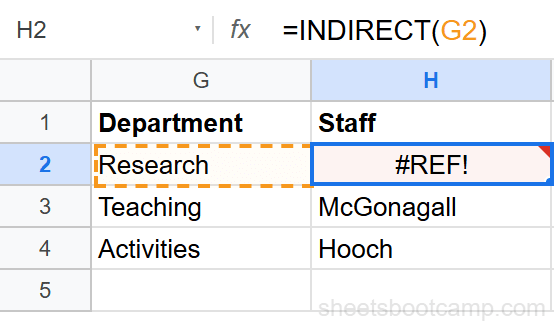
Check these three things:

1. Open Data > Named ranges and confirm the range exists.
2. Confirm the name matches the dropdown value exactly (spelling, no extra spaces).
3. If the dropdown shows a blank value in G2, INDIRECT has nothing to work with and will show #REF!.

Forgetting to Create Named Ranges Before Adding Validation

INDIRECT looks for named ranges at the time the dropdown opens. If you set up the H2 validation before creating the named ranges, the dropdown will show errors until the ranges exist. Create all named ranges first, then set the validation.

The Helper Cell Shows #REF! While the Department Cell Is Empty

If G2 is blank, =INDIRECT(G2) has no name to look up, so the helper cell shows #REF! and the Staff dropdown has nothing to offer. This is expected. It clears the moment a Department is selected. If you would rather not look at the error while the row is empty, wrap the helper: =IFERROR(INDIRECT(G2),"").

Tips

Each row needs its own helper. The dropdown rule points at a literal range like $N$2:$N$10, and that range is fed by one specific Department cell. Applying the same rule down H2:H100 does not give each row its own list: every row would show whatever G2 is currently driving. For a second row, add a second helper column, point it at G3, and give H3 a rule reading that column instead. This is the real cost of the technique, which is why it suits a small number of entry rows rather than a hundred.

Use VLOOKUP alongside dependent dropdowns. After the user selects a Department and Staff member, you can use VLOOKUP to pull additional data about that staff member from a reference table. For example: =VLOOKUP(H2, staff_table, 2, FALSE) retrieves their email address.

Pull reference lists from another file with IMPORTRANGE. If your department and staff lists live in a shared HR spreadsheet, use IMPORTRANGE to bring them into your working file. Create named ranges from the imported data so INDIRECT can find them.

Build 3-level cascading dropdowns. Dependent dropdowns are not limited to two levels. You can chain them: Region > Department > Staff. Each level uses INDIRECT to reference a named range populated by the level above. The setup becomes more involved, but the logic stays the same.

Keep the reference area on a hidden sheet. Once your named ranges are set up, you can hide the reference sheet to keep the interface clean. Named ranges continue to work even when the source sheet is hidden.

Related Google Sheets Tutorials

• Data Validation in Google Sheets: The complete guide to validation rules including dropdowns, checkboxes, number rules, and custom formulas
• Dropdown Lists in Google Sheets: How to create a basic dropdown from a list or a range before adding dependencies
• Checkboxes in Google Sheets: Use checkboxes alongside dropdowns to track completion status in the same row
• VLOOKUP in Google Sheets: Pull data based on a selected dropdown value to populate related fields automatically
• IMPORTRANGE in Google Sheets: Bring reference data from a separate spreadsheet so your dropdown source lists stay in one place

Frequently Asked Questions

How do I create a dependent dropdown in Google Sheets?

Create named ranges for each list of options. Then put =INDIRECT(G2) in a spare helper cell, where G2 holds the value from your first dropdown, and let it spill that list down the column. Point the second dropdown’s Cell range at the helper range, such as =$N$2:$N$10. Google Sheets rejects =INDIRECT(G2) typed directly into the validation box with the message “Please enter a valid range”, so the helper cell is what makes the technique work.

What does INDIRECT do in a dependent dropdown?

INDIRECT converts a text string into a cell or range reference. Placed in a helper cell, =INDIRECT(G2) reads the text in G2, finds the named range with that name, and spills that list into the column. The dropdown then reads the helper range, so changing G2 changes the options.

Why does my dependent dropdown show a #REF! error?

The named range doesn’t exist or the name doesn’t match exactly. If G2 contains ‘Research’ but you have no named range called ‘Research’, INDIRECT has nothing to reference and the helper cell shows #REF!. Check that every value in your first dropdown has a corresponding named range.

Can dependent dropdowns work across multiple sheets in Google Sheets?

Yes. Create your named ranges from a reference sheet, then use INDIRECT in your data validation on any other sheet. The named ranges work across the entire spreadsheet file, so the location of the source data does not affect how INDIRECT finds them.