Create a Drop-Down List in Google Sheets
Learn how to create a dropdown list in Google Sheets with data validation. Restrict input, reduce errors, and keep your data clean. Step-by-step guide.
Sheets Bootcamp
March 7, 2026
A dropdown list in Google Sheets restricts a cell to a predefined set of values, so users pick from a menu instead of typing freely. It’s one of the most used features in data validation, and it takes about two minutes to set up. We’ll cover how to create one from typed values or a cell range, how to edit it, and how to avoid the most common mistakes.
In This Guide
- Step-by-Step: Create a Dropdown List
- Dropdown from a Cell Range
- Edit or Remove a Dropdown
- Common Mistakes
- Tips
- Related Google Sheets Tutorials
- Frequently Asked Questions
Step-by-Step: Create a Dropdown List
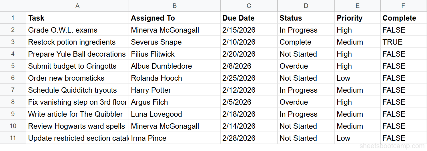
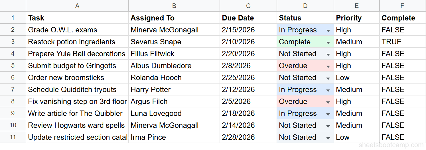
We’ll use a task tracker with ten rows of data. Column D holds the Status field, and we want to limit entries to four values: Not Started, In Progress, Complete, and Overdue.
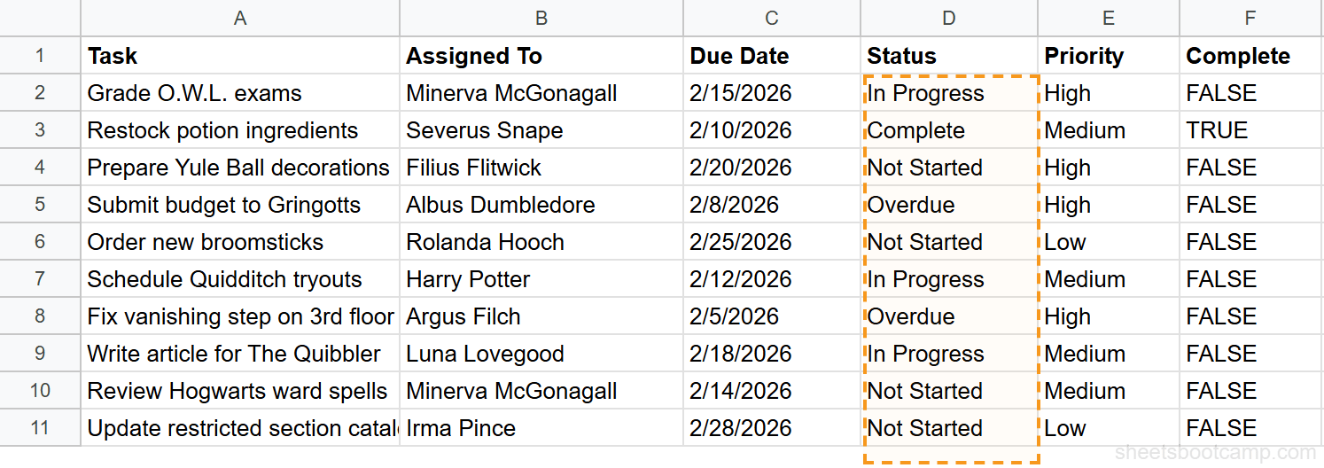
Select the cells for your dropdown
Select D2:D11. This covers all ten status cells in the task tracker. You can select more rows than you have data if you expect the list to grow. Selecting D2:D1000 works fine and costs nothing.
Open Data validation and choose Dropdown
Go to Data > Data validation in the top menu. A panel opens on the right side of the screen. Select Add rule. Under Criteria, open the dropdown and choose Dropdown. This mode accepts a manual list of values you type in.
Google Sheets updated the Data validation interface in 2023. If you see a dialog box instead of a side panel, you’re on an older version. The options are the same but arranged differently.
Enter your values and set rejection
Add each option as a separate entry:
- Not Started
- In Progress
- Complete
- Overdue
Under If the data is invalid, set it to Reject the input. This blocks users from typing anything outside the list. Without this setting, the dropdown shows a warning but still accepts the value. Select Done to apply the rule.
Set the behavior to Reject input, not Show warning. Show warning lets users bypass the list entirely. If the goal is data consistency, rejection is the right choice.
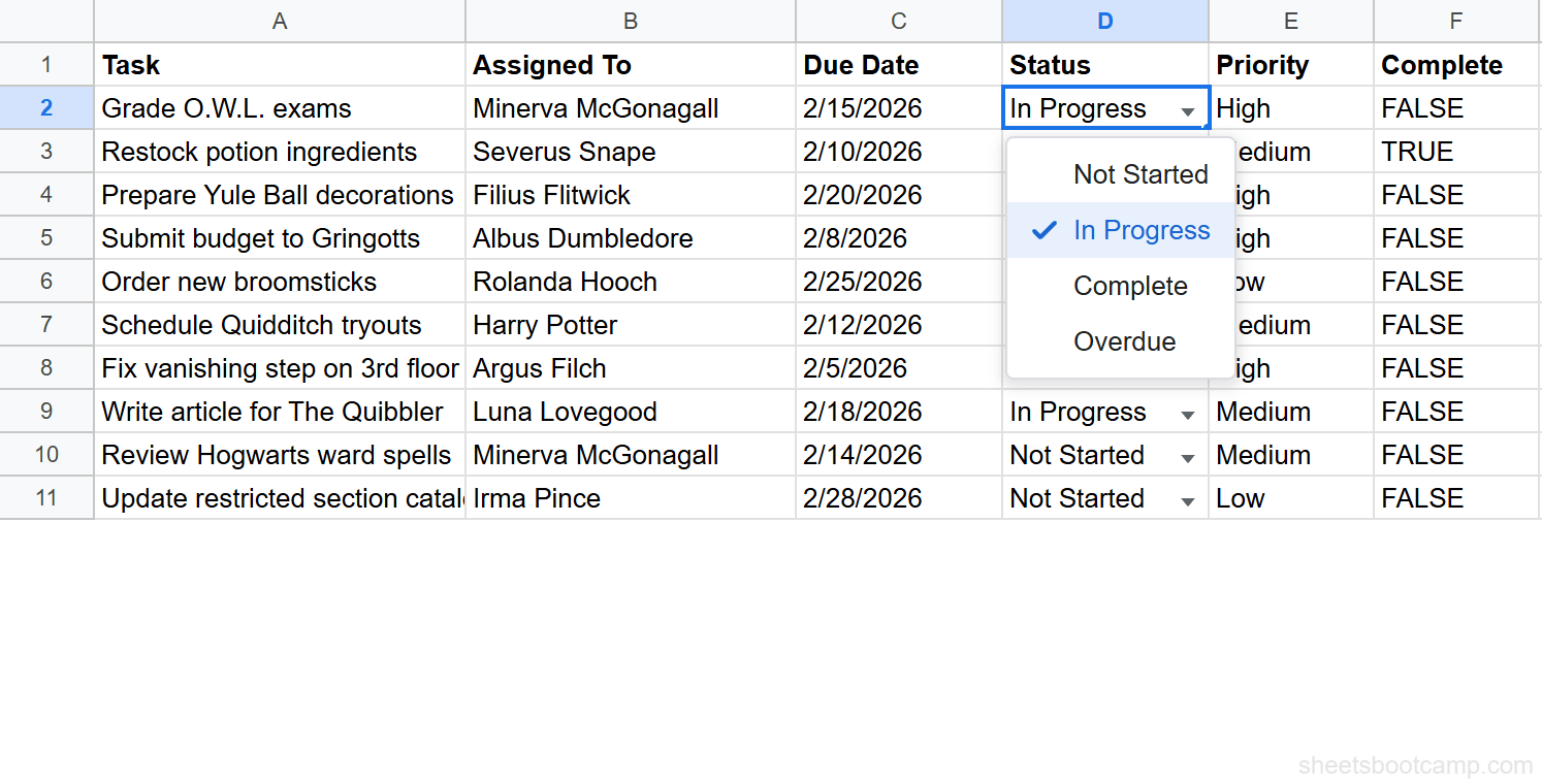
Test the dropdown
Select cell D2. A small arrow appears on the right edge of the cell. Select it to open the list. Pick any value and it fills the cell. Then try typing a value not in the list, such as “Pending.” Google Sheets displays a rejection message and reverts the cell.
Dropdown from a Cell Range
Typing values directly works well for short, stable lists. For longer lists or lists that change often, use a cell range as the source instead.
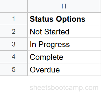
Create a reference list somewhere in your sheet. A common pattern is to use a column off to the right. In the example below, H1 contains the header “Status Options” and H2:H5 holds the four values.
To use this range as the dropdown source:
- Select D2:D11.
- Go to Data > Data validation > Add rule.
- Under Criteria, choose Dropdown (from a range).
- Enter
H2:H5in the range field, or select the cells directly. - Select Done.
The dropdown now pulls its options from column H. If you add a fifth status value to H6, you can update the range to H2:H6 and the dropdown reflects the change. You can also use a named range to make the reference easier to read.
Use UNIQUE to build a dynamic reference list from existing data. If your Status values already exist across many rows, =UNIQUE(D2:D100) in a helper column returns only the distinct values. Point your dropdown range there and it stays current automatically.
Edit or Remove a Dropdown
To edit a dropdown rule, select any cell in the validated range, then go to Data > Data validation. The panel shows the existing rule. Change the values, the range, or the rejection behavior, then select Done.
To delete the rule entirely, open Data > Data validation, find the rule, and select Remove rule. The cells return to unrestricted input. Any values already in those cells stay as they are. Users can now type anything without a warning.
Removing a validation rule does not clear cell contents. If D5 contained “Overdue” before you removed the rule, it still shows “Overdue” after. Only the input restriction is gone.
Common Mistakes
Extra spaces in your values
If you enter ” In Progress” with a leading space, the dropdown shows it with that space. Users who select it get a value that won’t match formulas expecting “In Progress”. Check each entry for leading and trailing spaces before saving the rule.
Using Show warning instead of Reject input
Show warning displays a tooltip when someone types an invalid value, but it still saves the entry. If you’re using the dropdown to feed a VLOOKUP or a COUNTIF, mismatched values silently break your formulas. Set it to Reject input when consistency matters.
Not extending the range for new rows
If your dropdown covers D2:D11 and you add row 12, the new cell has no validation. Either extend the rule to D2:D1000 upfront, or remember to update the rule when rows are added. The first approach is less error-prone.
Leaving the source range on the same sheet without protecting it
If your dropdown pulls from H2:H5, any user can accidentally overwrite those values and break the dropdown list. Consider putting the reference list on a separate sheet or using sheet protection on that range.
Tips
1. Assign colors to each option. In the Data validation panel, each dropdown value has a color chip next to it. Select the chip to assign a background color. “Overdue” in red and “Complete” in green makes status scanning much faster.
2. Combine with conditional formatting for row-level highlighting. A dropdown in column D can trigger a full-row color change in columns A through F. Set up a conditional formatting rule with a custom formula like =$D2="Overdue" applied to A2:F11. Every overdue row turns red automatically. For details, see conditional formatting with custom formulas.
3. Use COUNTIF to audit your data. After applying a dropdown, you can count how many tasks are in each status with:
=COUNTIF(D2:D11, "In Progress")This returns the count of cells in D2:D11 that match “In Progress” exactly. See COUNTIF in Google Sheets for more counting patterns.
4. Put the reference list on a dedicated sheet. A sheet named “Lists” keeps your reference data separate from working data. Name the range (e.g., StatusOptions) and reference it as Lists!A2:A5 in your validation rule. This prevents users from accidentally editing the source values.
5. Extend validation before you need it. If your data grows by one row per week, set the dropdown range to D2:D500 from the start. Google Sheets applies validation only to cells with content, so extra empty rows cost nothing.
Related Google Sheets Tutorials
- Data Validation in Google Sheets — The complete guide to restricting cell input with dates, numbers, text length, and custom formulas
- Dependent Dropdown Lists in Google Sheets — Make a second dropdown change its options based on what was selected in the first
- Checkboxes in Google Sheets — Add TRUE/FALSE checkboxes with a single click and use them in formulas
- Conditional Formatting in Google Sheets — Apply automatic color coding based on cell values, formulas, or date conditions
- VLOOKUP in Google Sheets — Pull related data from another table using the value selected in a dropdown cell
Frequently Asked Questions
How do I create a dropdown list in Google Sheets?
Select the cells where you want the dropdown, open Data > Data validation, choose Dropdown, enter your values separated by commas, and click Done. Each value appears as an option when users select a cell.
Can I create a dropdown list from a range of cells?
Yes. In the Data validation dialog, choose Dropdown (from a range) instead of Dropdown. Then select or enter the cell range that contains your list values, such as H2:H5. When you update the range, the dropdown updates automatically.
How do I edit or remove a dropdown list in Google Sheets?
Select the cells with the dropdown, open Data > Data validation, and modify or delete the rule. To remove the dropdown entirely, click Remove rule. Existing cell values remain but users can type anything without restriction.
Can I add colors to dropdown options in Google Sheets?
Yes. Google Sheets lets you assign a color to each dropdown option directly in the Data validation dialog. You can also use conditional formatting rules to apply background colors based on the selected value.