FLATTEN Function in Google Sheets

The FLATTEN function in Google Sheets converts a multi-column range into a single column. It reads across each row from left to right, then moves down to the next row, stacking every value vertically.

This is useful when you need to combine data from multiple columns into one list, feed it into another function like UNIQUE or SORT, or prepare data for charts that expect a single-column input.

In This Guide

• Syntax
• How to Use FLATTEN: Step-by-Step
• FLATTEN Examples
• Common Errors and How to Fix Them
• Tips and Best Practices
• Related Google Sheets Tutorials
• FAQ

Syntax

=FLATTEN(range1, [range2, ...])

FLATTEN accepts one or more ranges. Each range is read row by row from left to right, and the values are stacked into a single column.

How to Use FLATTEN: Step-by-Step

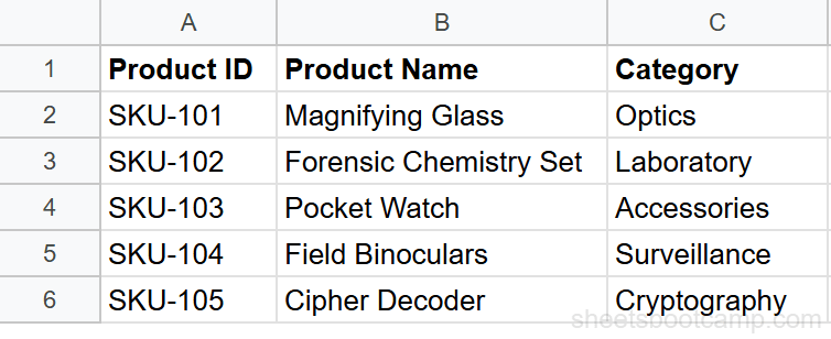
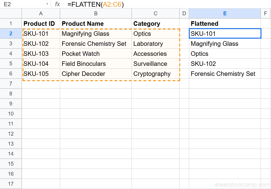
Here is a product inventory table with three columns of data in A2:C6.

Click cell E2 and enter:

=FLATTEN(A2:C6)

The result spills down into 15 rows (5 rows x 3 columns). Each row’s values appear in order: SKU-101, Magnifying Glass, Optics, SKU-102, Forensic Chemistry Set, Laboratory, and so on.

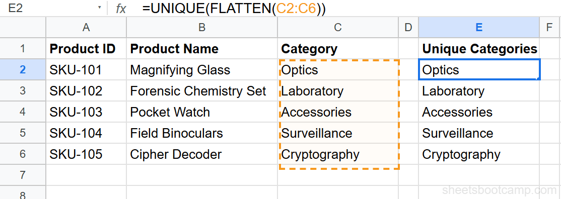
Wrap FLATTEN in UNIQUE to get a deduplicated list:

=UNIQUE(FLATTEN(C2:C6))

This returns each category once, even if the same category appears in multiple rows.

FLATTEN Examples

Flatten non-adjacent columns

To flatten only columns A and C (skipping B), use curly braces:

=FLATTEN({A2:A6, C2:C6})

This returns SKU-101, Optics, SKU-102, Laboratory, and so on. The curly braces create an array from the two ranges, and FLATTEN converts it to a single column.

Remove blanks from flattened output

FLATTEN includes empty cells as blank rows. To remove them, wrap the result in QUERY:

=QUERY(FLATTEN(A2:C10), "where Col1 is not null")

The QUERY function filters out blank rows, returning only cells with content.

Flatten and count unique values

Combine FLATTEN with UNIQUE and COUNTA to count how many distinct values exist across multiple columns:

=COUNTA(UNIQUE(FLATTEN(A2:C6)))

This returns a single number: the count of unique, non-blank values across the entire range.

Combine data from multiple sheets

Use FLATTEN with curly braces to combine ranges from different sheets:

=FLATTEN({Sheet1!A2:A10, Sheet2!A2:A10})

This stacks the values from column A of both sheets into one continuous list. Both ranges must have the same number of rows.

Common Errors and How to Fix Them

#REF! error

This happens when the flattened output does not have enough room to spill. The cells below the formula must be empty. Clear any data in the output area and try again.

Blank rows in the output

FLATTEN includes every cell in the range, including empty ones. If your source range extends beyond the data (e.g., A2:C100 but data only goes to row 20), the output has blank rows. Limit the range to your actual data, or filter blanks with QUERY.

Mixed data types

FLATTEN does not convert data types. If your range contains a mix of numbers, text, and dates, they all appear in the output column in their original format. This can cause issues if you feed the result into a function that expects uniform types.

Tips and Best Practices

1. Use FLATTEN to build dropdown source lists. Combine UNIQUE and FLATTEN to generate a deduplicated list from multiple columns, then reference it in a data validation dropdown.
2. Limit the input range. Flatten only the rows with data. Using open-ended ranges like A:C returns thousands of blank rows.
3. Combine with FILTER for conditional flattening. Flatten a range and then filter the result to keep only values that match a condition.
4. FLATTEN reads row by row. The order is left to right across each row, then down to the next row. If column order matters in your output, arrange the source range accordingly.
5. Use ARRAYFORMULA for transformations. If you need to modify every value in a flattened list (e.g., add a prefix), wrap the FLATTEN result in ARRAYFORMULA.

Related Google Sheets Tutorials

• UNIQUE Function — Remove duplicates from a flattened list
• SORT Function — Sort the output of FLATTEN alphabetically or numerically
• FILTER Function — Filter a flattened list based on conditions
• ARRAYFORMULA Guide — Apply transformations to every value in an array

FAQ

What does FLATTEN do in Google Sheets?

FLATTEN takes a multi-column or multi-row range and converts it into a single column. It reads the data left to right across each row, then moves to the next row. The result is a vertical list of every value in the range.

Is FLATTEN available in Excel?

No. FLATTEN is a Google Sheets-only function. In Excel, you can achieve a similar result using TOCOL (available in Microsoft 365) or a combination of INDEX and ROW formulas.

Does FLATTEN include blank cells?

Yes. FLATTEN includes empty cells from the range as blank rows in the output. To remove blanks, wrap it in QUERY: =QUERY(FLATTEN(A2:C6), "where Col1 is not null").

Can I FLATTEN non-adjacent ranges?

Yes. Use curly braces to combine ranges: =FLATTEN({A2:A6, C2:C6}). This flattens columns A and C while skipping column B. The ranges must have the same number of rows.

How do I get unique values from multiple columns?

Use =UNIQUE(FLATTEN(A2:C6)). FLATTEN combines all columns into one, then UNIQUE removes the duplicates. This is useful for building dropdown lists or summary reports from multi-column data.

What order does FLATTEN read the data?

FLATTEN reads left to right across each row, then moves to the next row. For a range A1:C3, the order is A1, B1, C1, A2, B2, C2, A3, B3, C3.