HYPERLINK Function in Google Sheets

The HYPERLINK function in Google Sheets creates a clickable link inside a cell. You give it a URL and display text, and it returns a blue, underlined link that opens the target when clicked.

This is useful when your spreadsheet has URLs in one column and you want clean, labeled links instead of raw addresses. HYPERLINK also works with email addresses, links to other sheets in the same file, and dynamically built URLs.

In This Guide

• Syntax
• How to Use HYPERLINK: Step-by-Step
• HYPERLINK Examples
• Common Errors and How to Fix Them
• Tips and Best Practices
• Related Google Sheets Tutorials
• FAQ

Syntax

=HYPERLINK(url, [link_label])

How to Use HYPERLINK: Step-by-Step

Click the cell where you want the link. Enter:

=HYPERLINK("https://example.com/product", "View Details")

Press Enter. The cell displays “View Details” in blue text.

Click the cell to see a tooltip with the URL. Click the link in the tooltip to open it in a new browser tab. The display text stays in the cell.

Instead of hardcoding the URL, reference a cell that contains it:

=HYPERLINK(D2, "View Details")

Now the link updates automatically whenever you change the URL in cell D2. This is useful when URLs are generated or imported from another source.

HYPERLINK Examples

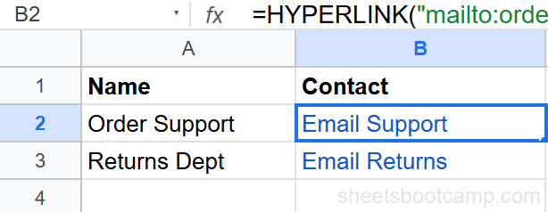
Link to an email address

=HYPERLINK("mailto:orders@example.com", "Email Support")

Clicking the link opens the default email client with the To field pre-filled. You can add a subject line: =HYPERLINK("mailto:orders@example.com?subject=Order Question", "Email Support").

Link to another sheet in the same spreadsheet

=HYPERLINK("#gid=0", "Go to Sheet1")

The #gid= format links to a specific sheet tab within the same spreadsheet. Find the gid by clicking the target sheet tab and checking the URL in your browser’s address bar. The number after gid= is the sheet ID.

Link to a specific cell in another sheet

=HYPERLINK("#gid=0&range=B5", "Jump to B5")

Adding &range=B5 to the gid link scrolls to and selects that cell when clicked. This is useful for navigation menus or table of contents sheets.

Build links dynamically from data

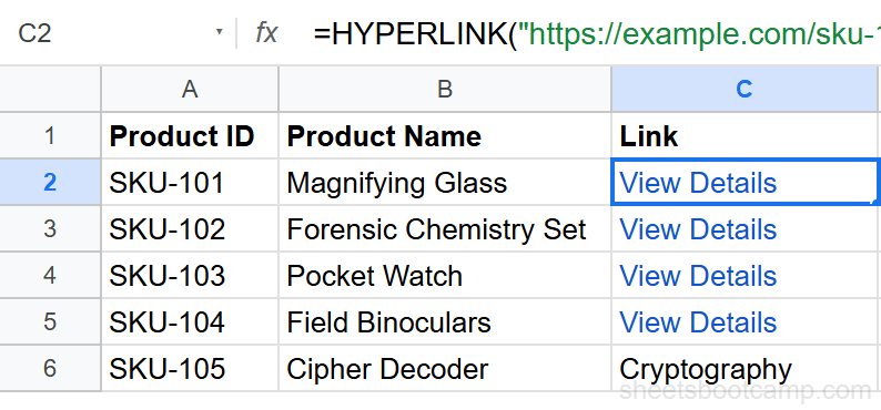
If column A has product IDs and you want each row to link to a product page:

=HYPERLINK("https://store.example.com/product/" & A2, B2)

This creates a link like https://store.example.com/product/SKU-101 with the product name from column B as the display text. Copy the formula down the column for every row.

Common Errors and How to Fix Them

Link shows the raw URL instead of display text

You omitted the second argument. Add display text as the second parameter: =HYPERLINK("https://example.com", "Click Here").

#VALUE! error

The URL argument is empty or the formula syntax has mismatched quotes. Check that both the opening and closing quotes around the URL are present.

Link does not open when clicked

Google Sheets links open via a tooltip that appears when you click the cell. Click the blue link in the tooltip popup, not the cell text itself. If the tooltip does not appear, the formula may have an error. Check the formula bar for issues.

Tips and Best Practices

1. Always include a link_label. Raw URLs in cells are hard to read and make your sheet look cluttered. A short label like “View” or “Open” is cleaner.
2. Use cell references for URLs that change. If the base URL or parameters might update, store the URL in a helper column and reference it in HYPERLINK.
3. Combine with VLOOKUP or INDEX MATCH for dynamic lookups. You can look up a URL from a reference table and wrap the result in HYPERLINK to create context-aware links.
4. Use HYPERLINK for navigation sheets. Build a “Dashboard” or “Table of Contents” sheet with HYPERLINK formulas linking to every other sheet in the workbook using #gid= URLs.
5. Links are preserved when you share the sheet. Anyone with access can click the links, whether they are viewing or editing.

Related Google Sheets Tutorials

• CONCATENATE and TEXTJOIN — Build dynamic URLs by combining text and cell values
• IMPORTRANGE in Google Sheets — Pull data from external spreadsheets into your sheet
• VLOOKUP in Google Sheets — Look up URLs or data to feed into HYPERLINK formulas
• How to Share Google Sheets — Share sheets with working hyperlinks to collaborators

FAQ

How do I add a hyperlink in Google Sheets?

Use the HYPERLINK function: =HYPERLINK("https://example.com", "Link Text"). The first argument is the URL, the second is the text shown in the cell. You can also right-click a cell and choose Insert link for a manual link.

Can HYPERLINK link to another sheet in the same spreadsheet?

Yes. Use the gid-based URL format: =HYPERLINK("#gid=0", "Go to Sheet1"). Find the gid by clicking the sheet tab and looking at the URL in your browser. The number after gid= is the sheet ID.

What is the difference between HYPERLINK and Insert link?

HYPERLINK is a formula, so the link updates dynamically if the URL cell changes. Insert link (right-click > Insert link) creates a static link attached to the cell. Use HYPERLINK when you need links that change based on data.

Can I create a mailto link with HYPERLINK?

Yes. Use =HYPERLINK("mailto:name@example.com", "Send Email"). Clicking the link opens the default email client with the To field pre-filled.

Why does my HYPERLINK show the URL instead of the display text?

If you omit the second argument, HYPERLINK displays the raw URL as the link text. Add a second argument for custom display text: =HYPERLINK(url, "Display Text").

Can I use HYPERLINK with VLOOKUP or other formulas?

Yes. You can nest formulas inside HYPERLINK. For example, =HYPERLINK(VLOOKUP(A2, Sheet2!A:B, 2, FALSE), "Open Link") looks up the URL from another sheet and turns it into a clickable link.